Wishocracy: Solving the Democratic Principal-Agent Problem Through Pairwise Preference Aggregation
Representative democracy suffers from an inescapable principal-agent problem where elected officials’ incentives diverge from citizen welfare. Wishocracy introduces RAPPA (Randomized Aggregated Pairwise Preference Allocation), which aggregates citizen preferences through cognitively tractable pairwise comparisons and creates accountability via Citizen Alignment Scores that channel electoral resources toward politicians who actually represent what citizens want.
Abstract
Politicians’ votes have near-zero correlation with citizen preferences (Gilens and Page, 2014). Elite preferences predict policy outcomes. No mechanism connects citizen preferences to electoral consequences for representatives.
RAPPA: Millions of citizens answer simple pairwise questions (“How would you split $100 between these two budget categories?”). Geometric mean aggregation produces population-level preference weights from sparse individual responses. Unlike approval voting or ranked choice, RAPPA captures preference intensity, not just what people want, but how much they care. Compare aggregated preferences to each legislator’s voting record. Publish Citizen Alignment Scores. Channel campaign resources to high-alignment candidates through Incentive Alignment Bonds.
The mechanism achieves three properties no prior system combines: minimal cognitive load (~20 comparisons per participant yields statistical convergence), preference intensity capture, and approximate strategy-proofness.
Keywords
mechanism design, principal-agent problem, collective intelligence, direct democracy, preference aggregation, participatory budgeting, analytic hierarchy process, public resource allocation
The Problem in One Sentence: Representative democracy suffers from an inescapable principal-agent problem: elected officials face incentives (re-election, donor pressure, special interests) that systematically diverge from citizen welfare, while direct democracy mechanisms are too cognitively demanding to scale beyond binary referenda.
The Solution: Wishocracy aggregates citizen preferences through simple pairwise comparisons (‘allocate $100 between cancer research and military spending’) and creates accountability for elected officials by publishing how their voting records align with these preferences. This channels electoral and financial resources toward politicians who actually represent what citizens want.
1 Abstract
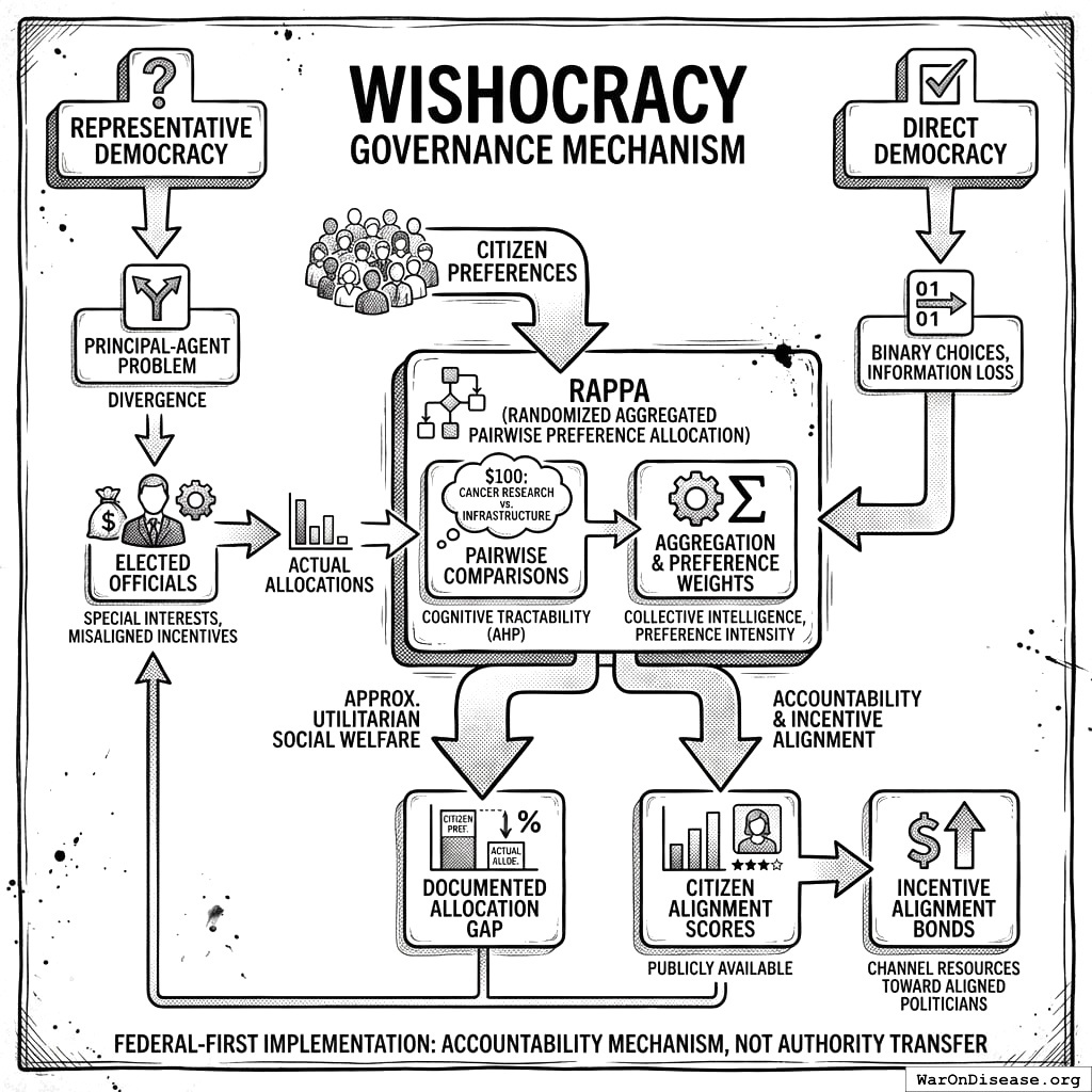
Representative democracy suffers from a fundamental principal-agent problem: elected officials systematically diverge from citizen preferences due to information asymmetry, special interest capture, and misaligned incentives. Meanwhile, direct democracy mechanisms reduce complex trade-offs to binary choices, losing crucial information about preference intensity. This paper introduces Wishocracy, a governance mechanism that addresses the democratic principal-agent problem by aggregating citizen preferences and creating accountability for elected representatives. The mechanism employs Randomized Aggregated Pairwise Preference Allocation (RAPPA), which presents participants with simple pairwise comparisons (‘allocate $100 between cancer research and infrastructure’) and aggregates millions of such judgments into preference weights that approximate utilitarian social welfare. Building on the Analytic Hierarchy Process133 for cognitive tractability and collective intelligence research134 for aggregation, RAPPA decomposes n-dimensional preference spaces into tractable binary choices while preserving preference intensity information. We present formal mechanism properties, computational complexity analysis, and empirical precedents from Porto Alegre’s participatory budgeting, Taiwan’s vTaiwan platform, and Stanford’s voting research. Rather than replacing representative democracy at the municipal level, we propose a federal-first implementation: (1) documenting the gap between citizen preferences and actual federal allocations, (2) creating public “Citizen Alignment Scores” for elected officials, and (3) integrating with Incentive Alignment Bonds to channel electoral and financial resources toward politicians whose voting records align with aggregated citizen preferences. This approach treats Wishocracy as an accountability mechanism that makes representative democracy work better, requiring no authority transfer, only information provision and incentive alignment.
2 Introduction: The Preference Aggregation Problem
Modern democracies face an increasingly acute challenge: how to translate the diverse, often conflicting preferences of millions of citizens into coherent public policy. Traditional electoral mechanisms were designed for an era of limited communication, discrete choices, and relatively homogeneous electorates. Today’s policy landscape (spanning healthcare allocation, infrastructure investment, climate adaptation, research funding, and social services) demands more sophisticated preference elicitation than periodic elections can provide.
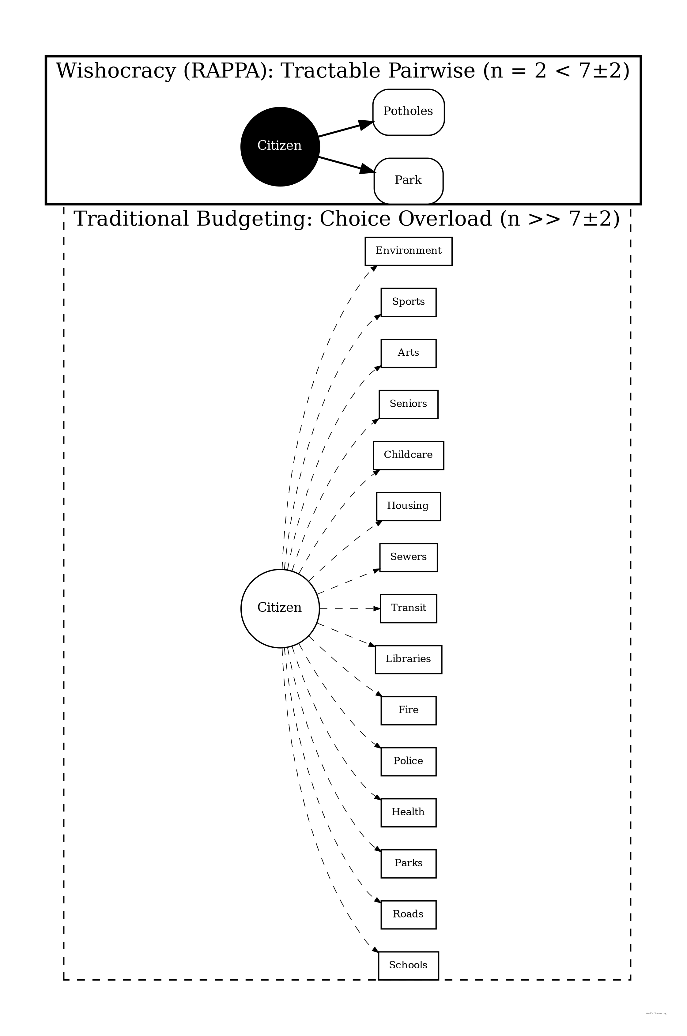
The fundamental problem is computational and cognitive. When citizens are asked to rank or rate dozens of competing priorities simultaneously, they face impossible cognitive demands. Research in behavioral economics has consistently demonstrated that humans cannot reliably compare more than 7±2 options simultaneously135. Humans struggle to make consistent judgments over large sets of options. Pairwise comparisons keep each decision local and cognitively manageable even when the full budget has thousands of items.
Yet modern government budgets allocate resources across thousands of line items, each representing implicit trade-offs against all others.
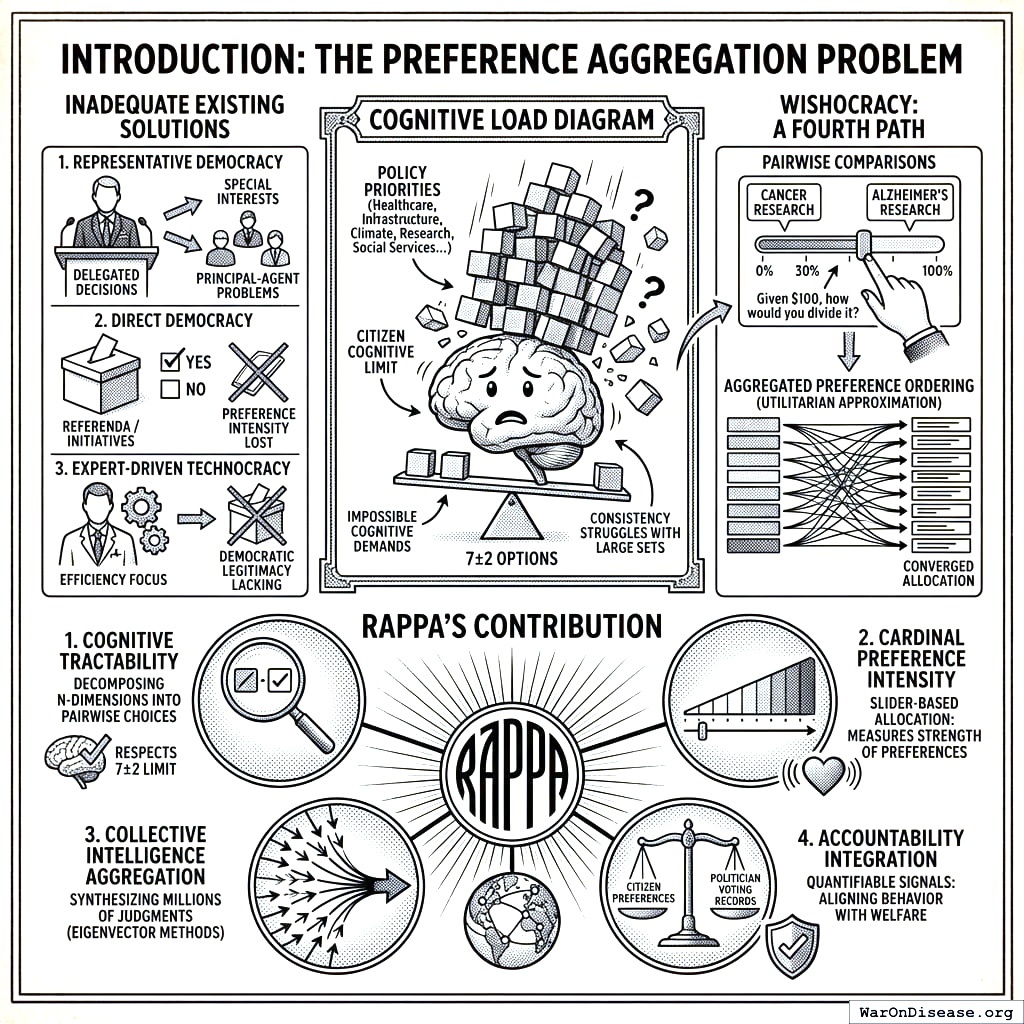
Existing solutions fall into three inadequate categories. First, representative democracy delegates preference aggregation to elected officials, introducing principal-agent problems, capture by special interests, and systematic misalignment between voter preferences and policy outcomes. Second, direct democracy mechanisms like referenda and citizen initiatives reduce complex trade-offs to binary choices, losing crucial information about preference intensity and creating winner-take-all dynamics that harm minorities with strong preferences. Third, expert-driven technocracy may achieve allocative efficiency but lacks democratic legitimacy and cannot incorporate the subjective welfare considerations that only citizens themselves can evaluate.
Wishocracy offers a fourth path: a mechanism that harnesses collective intelligence through structured preference elicitation while respecting cognitive constraints, incorporating preference intensity, and maintaining democratic legitimacy. By presenting citizens with simple pairwise comparisons (‘Given $100 to allocate between cancer research and Alzheimer’s research, how would you divide it?’), the mechanism decomposes the impossible n-dimensional comparison into tractable binary choices. Aggregated across millions of such comparisons from thousands of participants, the system converges on a preference ordering that approximates the utilitarian social welfare function under stated assumptions.
RAPPA’s Contribution: Wishocracy synthesizes four properties into a single framework:
Cognitive Tractability: By decomposing n-dimensional budget allocation into pairwise comparisons (drawing on AHP), RAPPA respects the well-documented cognitive limit of \(7 \pm 2\) simultaneous comparisons, making participation feasible for all citizens regardless of education or available time.
Cardinal Preference Intensity: Through slider-based allocation between pairs, participants reveal not just ordinal rankings but the strength of their preferences, allowing the mechanism to weight both the number of supporters and the intensity of their support.
Collective Intelligence Aggregation: By synthesizing millions of pairwise judgments through eigenvector methods, the mechanism uses diversity to cancel individual errors while aggregating true signals into allocations that approximate utilitarian social welfare.
Accountability Integration: By producing clear, quantifiable preference signals that can be compared against politician voting records, RAPPA enables accountability mechanisms (Citizen Alignment Scores, Incentive Alignment Bonds) that align representative behavior with citizen welfare.
To our knowledge, no widely deployed mechanism combines all four properties. Traditional voting captures neither intensity nor tractability. The Analytic Hierarchy Process provides tractability but has been deployed primarily for expert decision-making, not large-scale collective governance. Existing accountability mechanisms (interest group scorecards) reflect narrow priorities rather than aggregated citizen preferences. RAPPA synthesizes insights from decision science and collective intelligence to enable genuine democratic accountability.
3 Theoretical Foundations
3.1 The Analytic Hierarchy Process
Wishocracy’s methodological core derives from the Analytic Hierarchy Process (AHP), developed by Thomas Saaty at the Wharton School in the 1970s. AHP has been extensively validated across thousands of applications in business, engineering, healthcare, and government136. The method works because humans can reliably make pairwise comparisons even when direct multi-attribute rating fails.
AHP works by decomposing complex decisions into hierarchies of criteria and sub-criteria, then eliciting pairwise comparisons at each level. For n alternatives, this requires only n(n-1)/2 comparisons rather than the cognitively impossible simultaneous comparison of all n options. The pairwise comparison matrices are then synthesized using eigenvector methods to produce consistent priority rankings.
Crucially, AHP includes consistency checks through the calculation of a Consistency Ratio (CR). When individual judgments violate transitivity (e.g., A > B, B > C, but C > A), the method flags these inconsistencies for review. In Wishocracy’s collective aggregation, individual inconsistencies cancel out through the law of large numbers, while systematic collective preferences emerge from the aggregate.
3.2 The Preference Intensity Problem
A fundamental limitation of traditional voting is the failure to account for preference intensity. Under one-person-one-vote, a citizen who mildly prefers policy A has equal influence to one for whom policy A is existentially important. This leads to systematic welfare losses: intense minorities can be steamrolled by indifferent majorities, and the resulting allocations fail to maximize aggregate welfare.
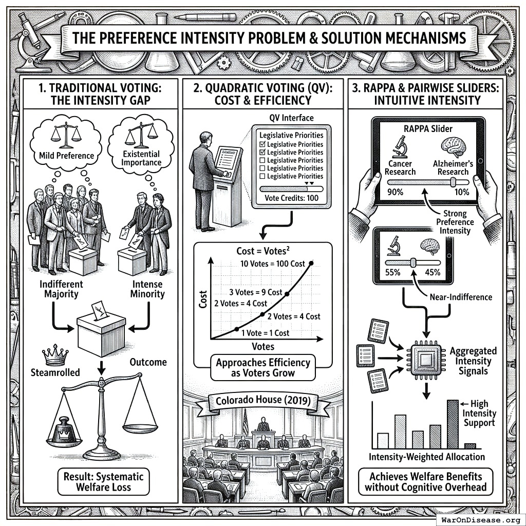
Several mechanisms have attempted to address this problem. Quadratic voting137 allows voters to purchase additional votes at quadratic cost, approaching efficiency as the number of voters grows. The Colorado House Democratic Caucus used QV in 2019 to prioritize legislative priorities. QV excels when voters face a manageable number of well-defined proposals. RAPPA addresses a complementary challenge: eliciting preferences across large, complex priority spaces where presenting all options simultaneously is infeasible. The two mechanisms can work in combination: RAPPA to identify and weight broad priorities through tractable pairwise comparisons, QV to allocate resources among specific proposals within those priorities.
RAPPA’s pairwise slider allocation captures preference intensity naturally. When a participant allocates 90% to cancer research and 10% to Alzheimer’s research, they express strong preference intensity. A 55-45 split signals near-indifference. This information emerges from intuitive trade-off judgments rather than strategic budget management. Aggregated across the population, these intensity signals produce allocations that weight both the number of supporters and the strength of their preferences, achieving the welfare benefits of intensity-weighted voting without the cognitive overhead.
3.3 Collective Intelligence and the Wisdom of Crowds
Wishocracy’s aggregation mechanism relies on the well-documented phenomenon of collective intelligence. Surowiecki134 synthesized research showing that diverse, independent groups consistently outperform individual experts under four conditions: diversity of opinion, independence of judgment, decentralization of information, and effective aggregation mechanisms.
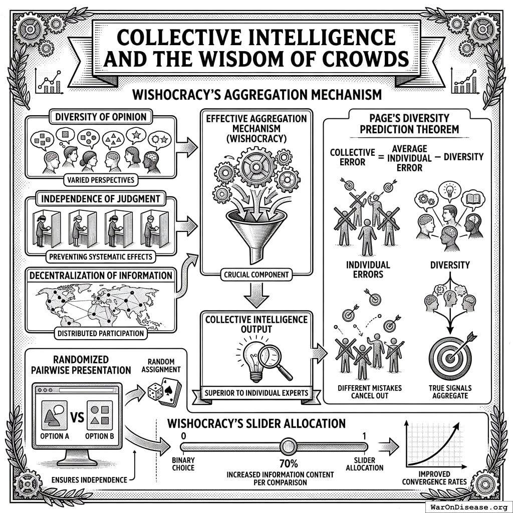
Randomized pairwise presentation ensures independence by preventing any systematic ordering effects. Diversity is maximized by including all citizens rather than restricting participation to experts or stakeholders. Decentralization emerges naturally from distributed participation. Wishocracy provides the crucial aggregation mechanism that previous collective intelligence applications have lacked.
Page’s diversity prediction theorem formalizes this intuition: collective error equals average individual error minus diversity. A diverse crowd makes different mistakes that cancel out, while sharing enough common knowledge that true signals aggregate. Wishocracy’s slider allocation (rather than binary choice) increases the information content per comparison, improving convergence rates.
3.4 Related Work and Positioning in the Literature
RAPPA exists within a broader landscape of democratic innovation and participatory governance mechanisms. We position Wishocracy relative to four major alternative approaches:
Liquid Democracy: Liquid democracy allows voters to either vote directly on issues or delegate their voting power to trusted representatives, with the ability to revoke delegation at any time. Examples include DelegativeVoting and Google’s internal Liquid Feedback experiments. While liquid democracy addresses representation flexibility, it does not solve the cognitive load problem: delegates still face the impossible task of ranking dozens of policy priorities simultaneously. RAPPA complements liquid democracy by providing a tractable preference elicitation method that delegates (or direct voters) can use.
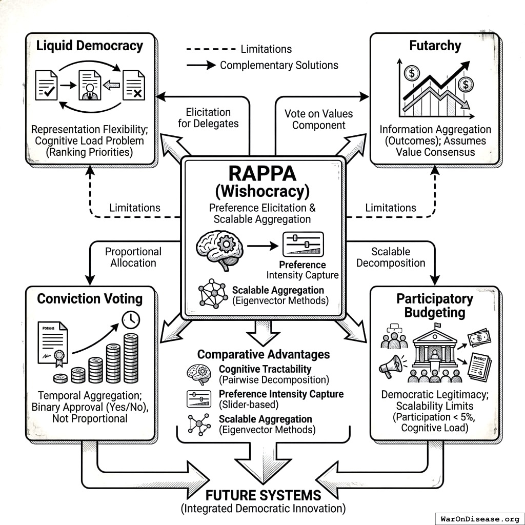
Futarchy: Proposed by economist Robin Hanson, futarchy uses prediction markets to aggregate information about which policies will best achieve agreed-upon goals. Under futarchy, “vote on values, bet on beliefs”: citizens determine welfare metrics democratically, then prediction markets determine which policies maximize those metrics. Futarchy excels at aggregating distributed information about causal mechanisms but assumes consensus on welfare metrics. RAPPA addresses the complementary problem: eliciting and aggregating preferences over competing welfare priorities when citizens disagree about relative importance (e.g., cancer research vs. education funding).
Conviction Voting: Used in decentralized autonomous organizations (DAOs), conviction voting allows continuous preference expression where tokens “accumulate conviction” on proposals over time. This mechanism rewards patience and sustained support while preventing sudden swings. However, conviction voting typically applies to binary proposal approval (fund this project: yes/no) rather than continuous budget allocation across competing priorities. RAPPA’s pairwise comparison approach enables proportional allocation that reflects both preference intensity and relative prioritization.
Participatory Budgeting: Traditional participatory budgeting (as pioneered in Porto Alegre138 and discussed in Section 4.1) involves citizen assemblies deliberating on budget proposals, followed by voting139. While highly democratic, this approach faces scalability limits: participation rates typically remain under 5%, and cognitive load increases exponentially with the number of budget items140. RAPPA retains participatory budgeting’s democratic legitimacy while achieving scalability through decomposition and statistical aggregation.
Comparative Advantages: RAPPA’s unique contribution lies in simultaneously addressing three constraints that limit alternative mechanisms: (1) Cognitive tractability through pairwise decomposition, (2) Preference intensity capture through slider-based allocation, and (3) Scalable aggregation through eigenvector methods that synthesize sparse distributed inputs. Where liquid democracy addresses who decides, futarchy addresses how to predict outcomes, and conviction voting addresses temporal aggregation, RAPPA addresses how to elicit preferences over complex multidimensional spaces.
This positioning suggests natural complementarities: RAPPA could serve as the preference elicitation layer for liquid democracy delegates, provide the “vote on values” component for futarchy systems, or replace binary voting in conviction voting contexts where proportional allocation is needed.
4 Mechanism Design: Randomized Aggregated Pairwise Preference Allocation
4.1 Core Mechanism
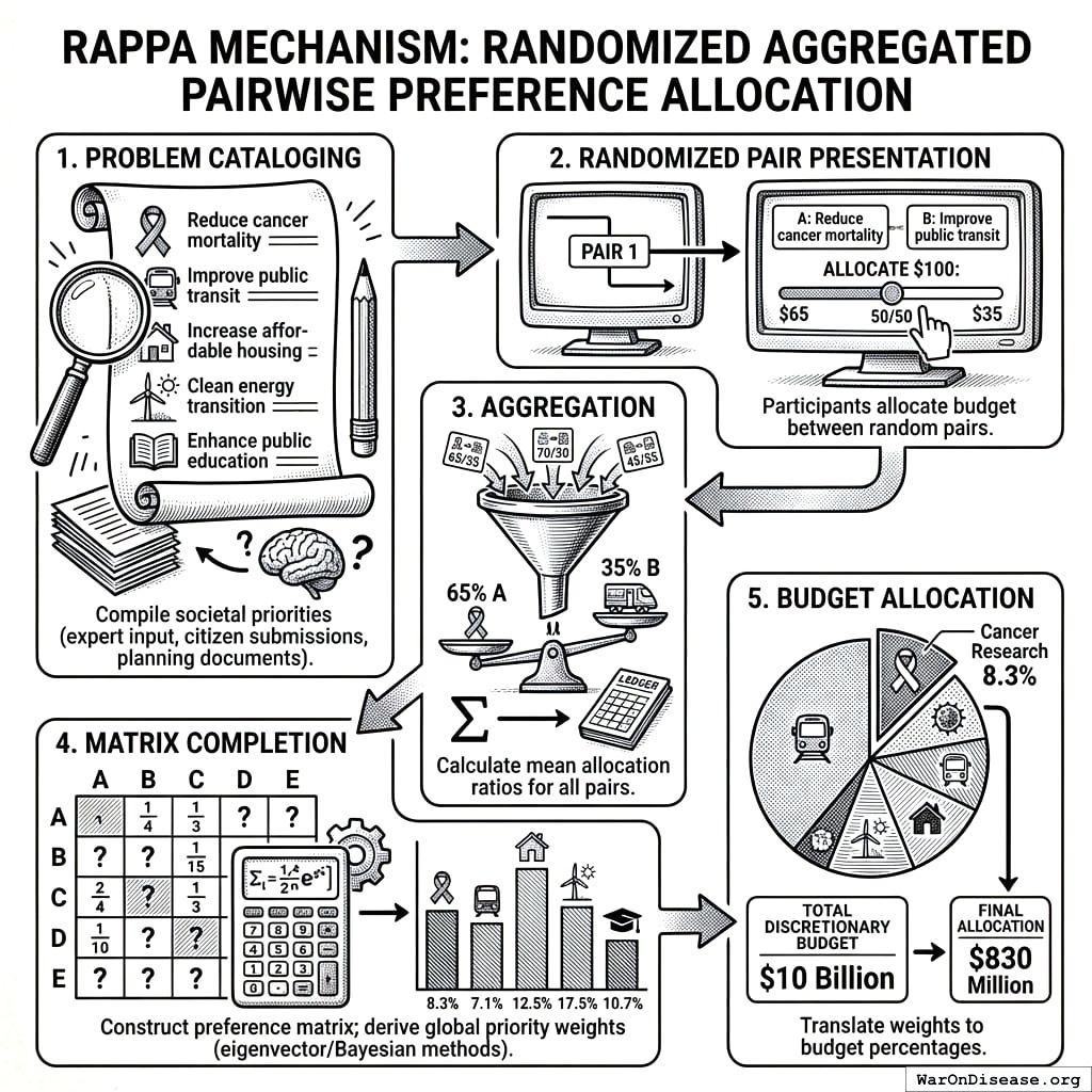
The Wishocracy mechanism operates through the following process, which we term Randomized Aggregated Pairwise Preference Allocation (RAPPA):
- Problem Cataloging: A comprehensive list of societal priorities, problems, or ‘wishes’ is compiled through expert input, citizen submissions, or existing government planning documents. These might include ‘Reduce cancer mortality,’ ‘Improve public transit,’ ‘Increase affordable housing,’ etc.
- Randomized Pair Presentation: Each participant is shown a series of randomly selected pairs from the problem catalog. For each pair, they are asked: ‘Given $100 to allocate between these two priorities, how would you divide it?’ A slider interface allows allocation anywhere from 100-0 to 0-100.
- Aggregation: All pairwise allocations are aggregated across participants. For each pair (A, B), the system calculates the mean allocation ratio. If participants on average allocate 65% to A and 35% to B, this establishes the relative priority weight.
- Matrix Completion: Using the aggregated pairwise ratios, a complete preference matrix is constructed. Standard eigenvector methods (as in AHP) or iterative Bayesian updating produce global priority weights for all n items.
- Budget Allocation: The final priority weights translate directly into budget allocation percentages. If cancer research receives a normalized weight of 8.3% and the total discretionary budget is $10 billion, cancer research receives $830 million.
4.1.1 Scenario: Federal Budget Preferences
Imagine Citizen Alice opening the Wishocracy app to express her preferences on federal spending.
- Comparison 1: She is presented with a pair: “Medical Research (NIH)” vs. “Military Weapons Systems”.
- Decision: Alice lost her mother to Alzheimer’s and believes medical research is severely underfunded. She slides the allocator to give 85% to Medical Research and 15% to Military. This expresses strong intensity.
- Comparison 2: Next, she sees “Military Weapons Systems” vs. “Drug Enforcement (DEA)”. She thinks both receive more than they should but slightly prefers maintaining military capability. She allocates 60% to Military and 40% to Drug Enforcement.
- Aggregation: Millions of other citizens make similar pairwise comparisons. Alice never sees “Medical Research vs. Drug Enforcement,” but the system infers the relationship (Medical Research > Military > Drug Enforcement) through the transitive network of all citizens’ choices.
- Result: The aggregate preferences reveal that citizens would allocate significantly more to medical research and less to military and drug enforcement than Congress currently does. This “Preference Gap” becomes the basis for Citizen Alignment Scores: politicians who vote to increase NIH funding score higher; those who vote for military expansion despite citizen preferences score lower.
4.2 Formal Properties
RAPPA satisfies several desirable mechanism design properties:
Pareto-Respecting (Discussion): The mechanism aims to produce allocations where no reallocation could make some participants better off without making others worse off, though formal proof depends on specific utility assumptions.
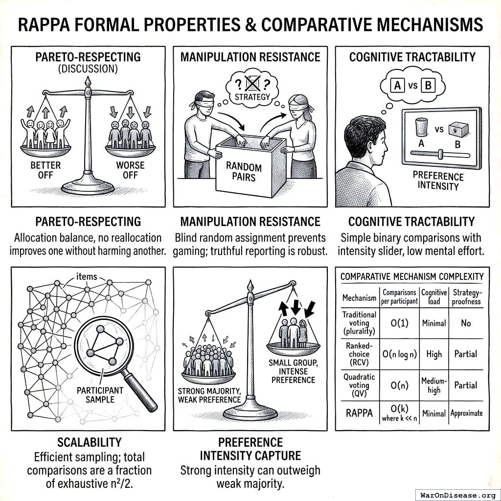
Manipulation Resistance: Random pair assignment makes strategic manipulation difficult. A participant cannot know which pairs they will receive, making truthful reporting a robust heuristic. With sufficiently large participant pools, individual strategic behavior has negligible impact on outcomes.
Cognitive Tractability: Each individual comparison requires only binary evaluation with an intensity slider, well within human cognitive capacity. Participants need not understand the aggregation mathematics.
Scalability: The number of pairwise comparisons grows quadratically with items (n²/2), but each participant need only complete a small random sample. Statistical convergence requires far fewer total comparisons than exhaustive coverage.
Preference Intensity Capture: Unlike binary voting, the slider allocation captures cardinal preferences. Strong majorities with weak preferences can be outweighed by smaller groups with intense preferences, addressing the tyranny of the majority problem.
Complementary Mechanisms: Different voting mechanisms excel in different contexts. The table below summarizes when each is best suited:
| Mechanism | Strengths | Best suited for |
|---|---|---|
| Traditional voting | Simple, universally understood, fast | Binary decisions, final ratification |
| Ranked-choice (RCV) | Eliminates spoiler effect, finds consensus | Single-winner elections among candidates |
| Quadratic voting (QV) | Reveals preference intensity, budget-like allocation | Prioritizing among well-defined proposals |
| RAPPA | Decomposes large option spaces into tractable comparisons | Preference discovery across many alternatives |
These mechanisms form a complementary toolkit. A governance system might use RAPPA to surface priorities across a large policy space, QV to allocate resources within categories, and traditional voting for final ratification.
4.3 Formal Model
We now formally define the RAPPA mechanism as a mapping from individual preferences to collective allocations.
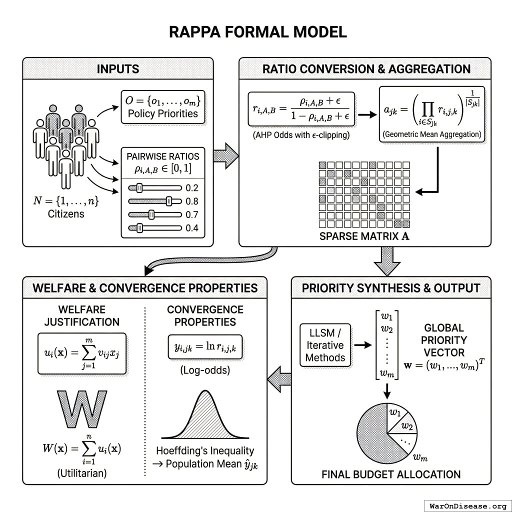
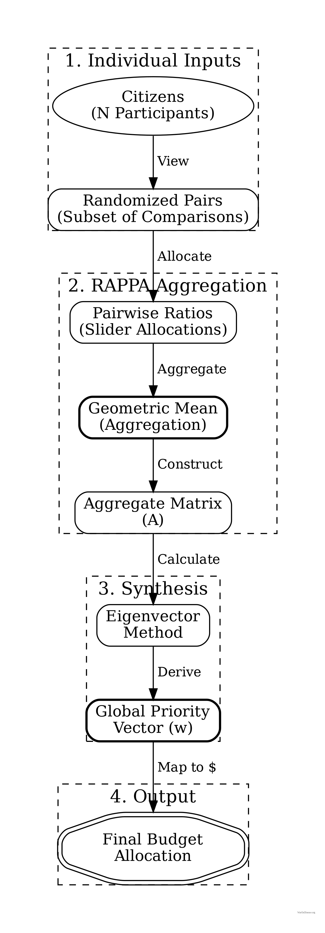
Inputs: Let \(N = \{1, ..., n\}\) be the set of citizens and \(O = \{o_1, ..., o_m\}\) be the set of policy priorities. Each citizen \(i\) provides pairwise allocation ratios \(\rho_{i,A,B} \in [0,1]\) for a subset of pairs \((A,B) \in O \times O\).
Ratio Conversion: The raw slider value \(\rho\) (a share) is converted into a preference odds ratio \(r\) (unbounded \([0, \infty)\)) to satisfy AHP requirements. We apply \(\epsilon\)-clipping to handle edge cases (0/100): \[ r_{i,A,B} = \frac{\rho_{i,A,B} + \epsilon}{1 - \rho_{i,A,B} + \epsilon} \] where \(\epsilon\) is a small constant (e.g., \(10^{-3}\)) to prevent singularities.
Aggregation Function: For each pair \((o_j, o_k)\), we compute the aggregate pairwise comparison using the Geometric Mean of individual odds ratios (following141, which proves geometric mean is necessary to preserve the reciprocal property in pairwise comparisons): \[ a_{jk} = \left( \prod_{i \in S_{jk}} r_{i,j,k} \right)^{\frac{1}{|S_{jk}|}} \]
Note: While we use geometric mean to aggregate individual pairwise comparisons (to preserve reciprocity), the resulting eigenvector priority weights approximate the arithmetic mean of individual utilities under appropriate conditions (see133 for details). where \(S_{jk} \subseteq N\) is the set of citizens who evaluated the pair. This produces a sparse \(m \times m\) comparison matrix \(\mathbf{A}\).
Priority Synthesis: We compute priorities from the sparse matrix \(\mathbf{A}\). While classical AHP uses the principal eigenvector of a dense matrix, for sparse data we employ logarithmic least squares (LLSM) or iterative methods to recover the global priority vector \(\mathbf{w} = (w_1, ..., w_m)^T\) such that \(a_{jk} \approx w_j / w_k\).
Output: The final budget allocation assigns fraction \(w_j\) of total resources to priority \(o_j\).
Welfare Justification: Under quasi-linear preferences where citizen \(i\)’s utility from allocation \(\mathbf{x} = (x_1, ..., x_m)\) is \(u_i(\mathbf{x}) = \sum_{j=1}^{m} v_{ij} x_j\), the pairwise allocation \(\rho_{i,j,k}\) reveals the relative valuations \(v_{ij}/v_{ik}\). The eigenvector aggregation produces weights \(w_j\) proportional to \(\sum_{i \in N} v_{ij}\), thus approximating the utilitarian welfare function \(W(\mathbf{x}) = \sum_{i=1}^{n} u_i(\mathbf{x})\) under budget constraint \(\sum_{j} x_j = B\).
Convergence Properties: Define the log-odds ratio \(y_{i,jk} = \ln r_{i,j,k}\). With \(\epsilon\)-clipping, \(y\) is bounded in \([\ln \epsilon - \ln(1+\epsilon), \ln(1+\epsilon) - \ln \epsilon]\). The aggregate estimator \(\hat{y}_{jk} = \frac{1}{|S_{jk}|} \sum_{i \in S_{jk}} y_{i,jk}\) concentrates around the population mean by Hoeffding’s inequality. The final aggregate ratio is \(a_{jk} = \exp(\hat{y}_{jk})\).
Wishocracy implies a separation of concerns: RAPPA determines what society values (the priority vector \(\mathbf{w}\)), while the implementation of those priorities is handled by a separate layer of competitive problem-solving organizations (see Appendix A: The Solution Layer). This distinction prevents the mechanism from bogging down in technical debates during the preference aggregation phase.
4.4 Computational Complexity and Scalability
We now analyze the computational requirements of RAPPA and establish scalability bounds for real-world deployment.
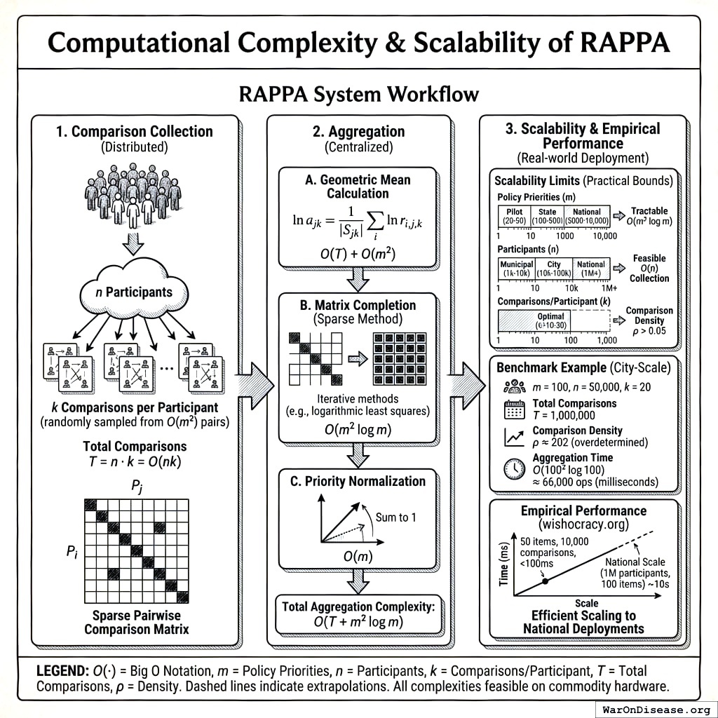
Comparison Collection Complexity: For \(m\) policy priorities, the complete pairwise comparison space contains \(\binom{m}{2} = \frac{m(m-1)}{2} = O(m^2)\) unique pairs. However, RAPPA employs random sampling rather than exhaustive coverage. Each of \(n\) participants completes \(k\) comparisons, yielding total comparison count \(T = n \cdot k = O(nk)\). \(k\) can be held constant (e.g., \(k=20\) comparisons per participant) regardless of \(m\), making per-participant complexity \(O(1)\) rather than \(O(m^2)\).
Aggregation Complexity: Given \(T\) collected comparisons distributed across \(O(m^2)\) possible pairs, aggregation proceeds in three steps:
Geometric mean calculation: For each observed pair \((j,k)\), compute geometric mean of \(|S_{jk}|\) individual ratios141. Using log transformation: \(\ln a_{jk} = \frac{1}{|S_{jk}|} \sum_{i \in S_{jk}} \ln r_{i,j,k}\). Complexity: \(O(T)\) for summing all comparisons, then \(O(m^2)\) for averaging pairs.
Matrix completion: Convert sparse observations into \(m \times m\) matrix \(\mathbf{A}\). For dense eigenvector methods (classical AHP133), this requires \(O(m^3)\) operations for eigendecomposition. For sparse data, iterative methods (e.g., logarithmic least squares, coordinate descent) converge in \(O(m^2 \log m)\) operations given sufficient comparison density.
Priority normalization: Normalize eigenvector to sum to 1. Complexity: \(O(m)\).
Total system complexity: \(O(nk + m^2 \log m)\) where the first term dominates for large-scale deployments (\(n \gg m\)).
Scalability Limits: Real-world constraints impose practical bounds:
Policy priorities (\(m\)): Pilot deployments (municipal budgets): \(m = 20-50\) items. State/national budgets: \(m = 100-500\) items. Full government budget line items: \(m = 5,000-10,000\) items. The \(O(m^2 \log m)\) aggregation complexity remains tractable even at \(m=10,000\) (requiring ~10^9 operations, feasible on commodity hardware in seconds).
Participants (\(n\)): Municipal scale: \(n = 1,000-10,000\) participants. City scale: \(n = 10,000-100,000\). National scale: \(n = 1,000,000+\). The linear \(O(n)\) scaling in comparison collection makes national-scale deployment computationally feasible.
Comparisons per participant (\(k\)): Empirical testing at wishocracy.org142 suggests \(k=10-30\) comparisons provides good user experience (5-10 minutes) while achieving convergence. Comparison density \(\rho = \frac{nk}{m(m-1)/2}\) should exceed \(\rho > 0.05\) for reliable estimates, implying minimum \(nk > 0.025m^2\) or equivalently \(n > 0.025m^2/k\).
Benchmark Example (City-Scale Deployment): Consider a city budget with \(m=100\) priorities, \(n=50,000\) participants, \(k=20\) comparisons each:
- Total comparisons: \(T = 50,000 \times 20 = 1,000,000\)
- Comparison density: \(\rho = \frac{1,000,000}{100 \times 99 / 2} = \frac{1,000,000}{4,950} \approx 202\) (highly overdetermined)
- Aggregation time: \(O(100^2 \log 100) \approx 66,000\) operations (milliseconds on modern hardware)
- Storage: \(O(m^2) = 10,000\) matrix entries (kilobytes)
This analysis demonstrates that RAPPA scales efficiently to city and even national deployments with commodity computing infrastructure. The sparse, distributed nature of data collection combined with efficient matrix completion algorithms makes the mechanism computationally tractable across all realistic governance scales.
Empirical Performance: The reference implementation at wishocracy.org142 processes 10,000 comparisons across 50 items in under 100ms on standard cloud infrastructure (AWS t3.medium instance). Extrapolating linearly, national-scale deployment (1M participants, 100 items) would require ~10 seconds of aggregation time, negligible compared to voting/deliberation timescales measured in days or weeks.
4.5 Comparative Information & Welfare Analysis
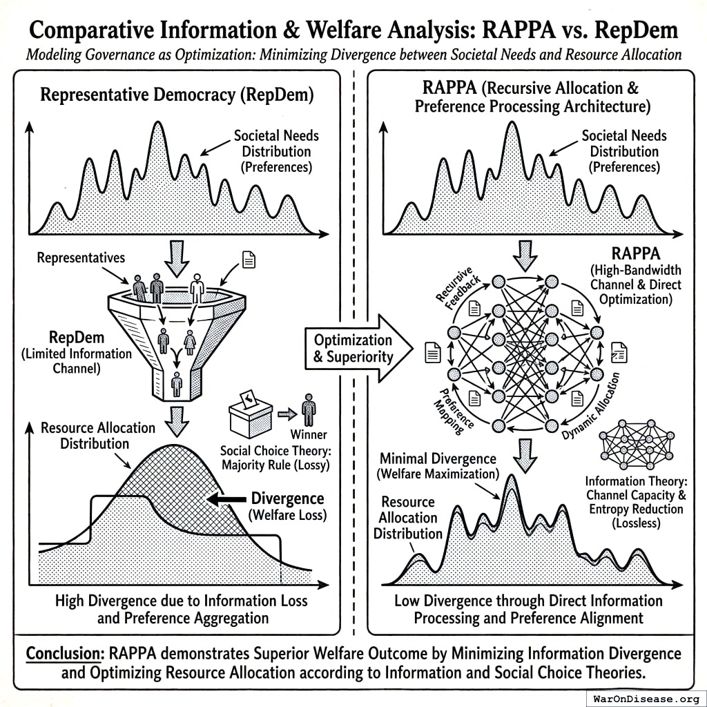
We now formally demonstrate the superiority of RAPPA over Representative Democracy (RepDem) using Information Theory and Social Choice Theory. We model governance as an optimization process where the objective is to minimize the divergence between the distribution of societal needs (preferences) and the distribution of resource allocation.
4.5.1 Information-Theoretic Superiority
Governance can be modeled as a source coding problem. Let \(\mathcal{P}\) be the true distribution of societal preferences over \(m\) issues. The mechanism must encode \(\mathcal{P}\) into a signal transmitted to the allocation engine.
Representative Democracy (Low-Bandwidth Channel):
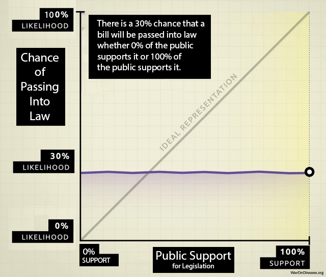
In RepDem, a voter transmits a single scalar signal \(v \in \{c_1, \dots, c_k\}\) (choosing one of \(k\) candidates) every \(T\) years. The channel capacity \(C_{Rep}\) is severely limited by quantization noise. A voter with a precise preference vector \(\vec{p} \in \mathbb{R}^m\) must compress this into a single nominal vote. \[ C_{Rep} \approx \frac{\log_2(k)}{T \text{ years}} \approx 0 \] This extreme lossy compression effectively destroys all information about preference intensity and specific trade-offs (The “Bundle Problem”). This theoretical result aligns with empirical findings by143, who analyzed 1,779 policy outcomes and found that “average citizens have little or no independent influence” on policy.
Wishocracy (High-Bandwidth Channel):
RAPPA operates as a continuous channel. Each pairwise comparison extracts \(\log_2(\text{resolution})\) bits of information about the relative valuation of outcome bundle subsets. With continuous sliders, the transmission rate is limited only by citizen engagement time. \[ C_{RAPPA} \propto N \cdot \bar{c} \cdot H(S) \] where \(N\) is voters, \(\bar{c}\) is average comparisons per voter, and \(H(S)\) is the entropy of the slider input.
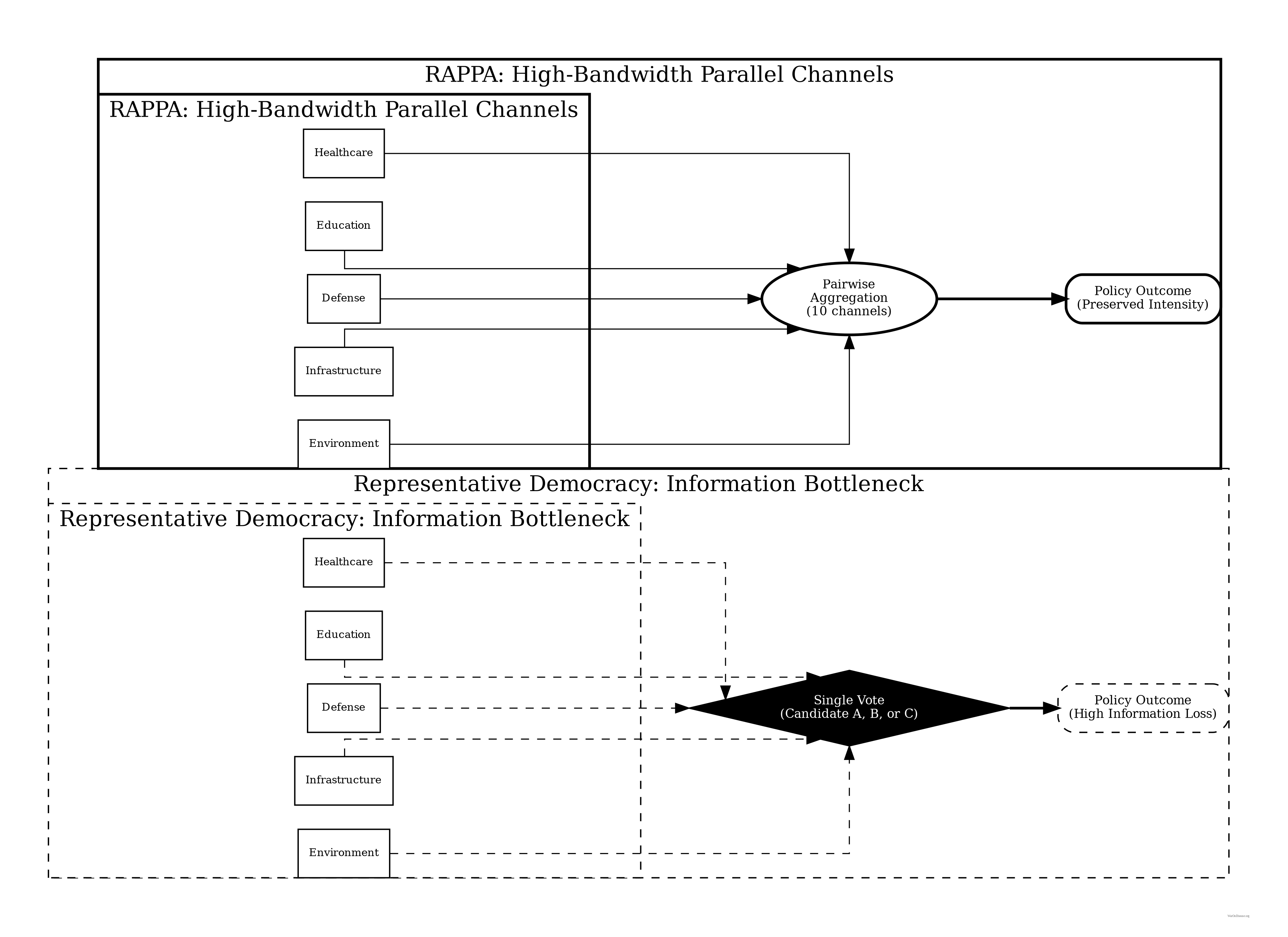
Proposition 1 (Information Loss in Candidate Voting): Let \(D_{KL}(P || Q)\) be the Kullback-Leibler divergence between true welfare preferences \(P\) and enacted policy \(Q\). As \(N \to \infty\): \[ E[D_{KL}(P || Q_{RAPPA})] \ll E[D_{KL}(P || Q_{Rep})] \] Argument (Sketch): By the Data Processing Inequality, post-processing (policymaking) cannot increase information. \(Q_{Rep}\) is derived from a signal with near-zero mutual information \(I(P; V_{Rep})\) due to quantization. \(Q_{RAPPA}\) is derived from a sufficient statistic of the pairwise matrix \(\mathbf{A}\), where \(I(P; \mathbf{A})\) approaches \(H(P)\) as empirical sampling density increases.
4.5.2 Welfare Maximization: The “Median vs. Mean” Proof
A fundamental result in Public Choice Theory is the Median Voter Theorem144, which states that under majority rule, outcomes converge to the preferences of the median voter, \(v_{median}\).
The Skewness Problem: In healthcare and public risk, damage distributions are highly right-skewed (power laws). A few citizens suffer catastrophic loss (e.g., rare diseases, pandemics), while the majority experiences zero loss.
- Median Outcome: If 51% of voters have priority \(x=0\) (healthy) and 49% have priority \(x=100\) (dying), the median preference is \(0\). The minority receives no aid.
- Mean Outcome: The utilitarian optimum is \(\bar{x} = 0.49 \times 100 = 49\).
Proposition 2 (Tail-Risk Under Median Aggregation): For any utility distribution \(U\) with skewness \(\gamma > 0\) (typical of health/wealth distributions), the Social Welfare \(W\) of the RAPPA allocation exceeds that of the Median Voter allocation. \[ W(RAPPA) \approx W(\text{Mean}) > W(\text{Median}) \] Argument: The RAPPA eigenvector centrality \(w_j\) corresponds to \(\frac{\sum v_{ij}}{\sum \sum v_{ik}}\), which approximates the population arithmetic mean. For convex loss functions (where distinct needs exist), minimizing the sum of squared errors leads to the mean, not the median. Wishocracy thus passes the “Veil of Ignorance” test145 whereby a citizen typically prefers the Mean allocation to the Median allocation to hedge against being in the tail risk category.
4.5.3 Principal-Agent Cost Elimination
Total Governance Loss \(L_{Gov}\) can be decomposed into Aggregation Loss (failure to aggregate preferences) and Agency Loss (corruption/misalignment).
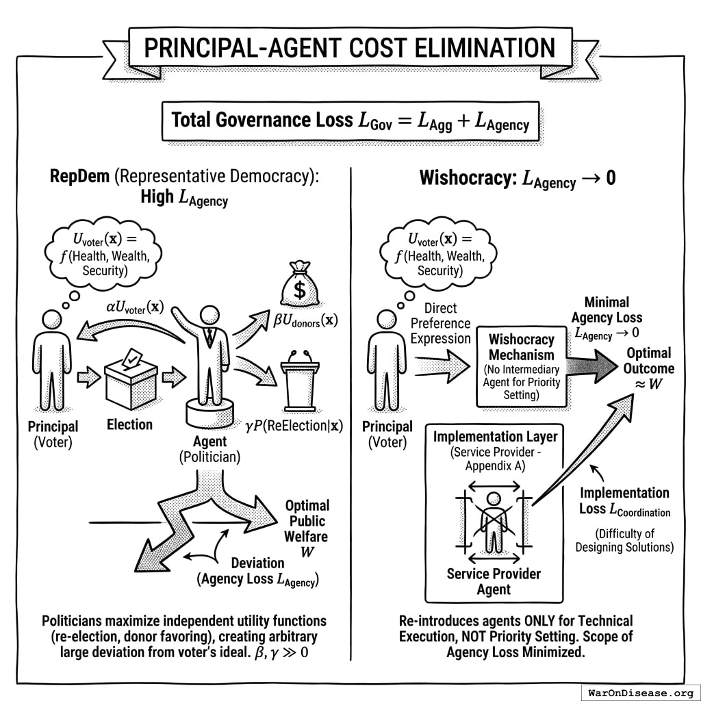
\[ L_{Gov} = L_{Agg} + L_{Agency} \]
- RepDem: suffer from high \(L_{Agency}\). Politicians maximize independent utility functions (re-election, donor favoring) rather than \(W\). Deviation can be arbitrarily large.
Formally, let the voter’s utility be \(U_{voter}(\mathbf{x}) = f(\text{Health}, \text{Wealth}, \text{Security})\) over allocation \(\mathbf{x}\). The politician’s utility is:
\[ U_{pol}(\mathbf{x}) = \alpha U_{voter}(\mathbf{x}) + \beta U_{donors}(\mathbf{x}) + \gamma P(\text{ReElection} | \mathbf{x}) \]
where \(\beta, \gamma \gg 0\). Since donor interests (\(U_{donors}\)) often conflict with public welfare (\(U_{voter}\)) (e.g., lower regulation vs. clean air), and re-election depends on short-term signaling rather than long-term outcomes, \(\text{argmax}(U_{pol}) \neq \text{argmax}(U_{voter})\).
- Wishocracy: \(L_{Agency} \to 0\). The mechanism is direct; there is no agent to bribe.
- Constraint: Wishocracy introduces \(L_{Coordination}\) (the difficulty of designing solutions), which is why the service provider layer (Appendix A) re-introduces agents only for implementation, not for priority setting, minimizing the scope of potential agency loss to technical execution rather than value judgment.
5 Empirical Precedents and Evidence Base
5.1 Porto Alegre Participatory Budgeting
The closest large-scale precedent for Wishocracy is participatory budgeting (PB), pioneered in Porto Alegre, Brazil in 1989. Under the Workers’ Party administration, citizens were invited to deliberative assemblies to determine municipal investment priorities. By 1997, PB produced remarkable results: sewer and water connections increased from 75% to 98% of households; health and education budgets grew from 13% to 40% of total spending; the number of schools quadrupled; and road construction in poor neighborhoods increased five-fold.
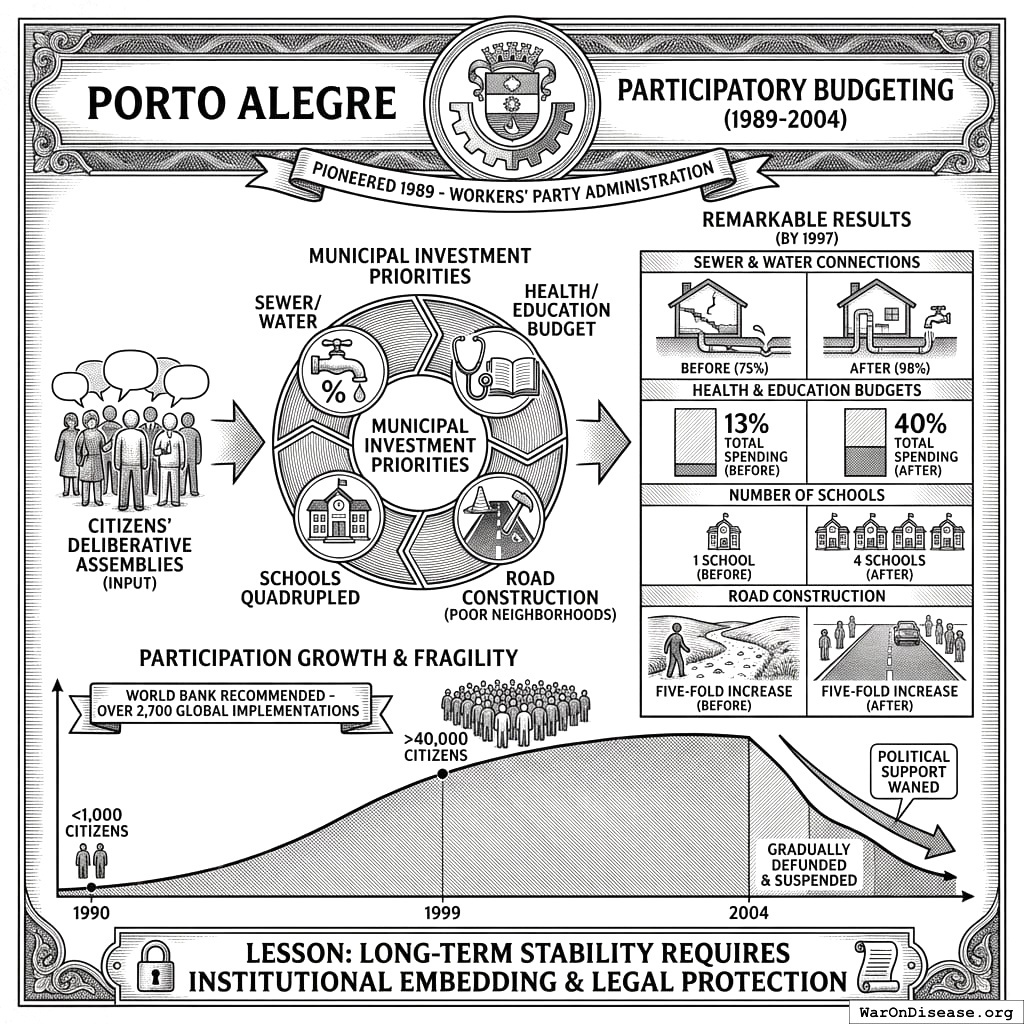
Participation grew from fewer than 1,000 citizens annually in 1990 to over 40,000 by 1999. The World Bank documented PB’s success in improving service delivery to the poor and has since recommended its adoption worldwide. Over 2,700 governments have implemented some form of participatory budgeting.
However, Porto Alegre also illustrates the fragility of participatory mechanisms. When political support waned after 2004, PB was gradually defunded and eventually suspended. This underscores the importance of institutional embedding and legal protection for any participatory mechanism seeking long-term stability.
5.2 Taiwan’s Digital Democracy Experiments
Taiwan’s vTaiwan platform, launched in 2014 by civic hacker Audrey Tang (later Taiwan’s Digital Minister), demonstrates the potential of technology-mediated preference aggregation. The platform used Pol.is, a tool that maps opinions and identifies consensus clusters, to deliberate on contentious policy issues including ridesharing regulation and online alcohol sales.
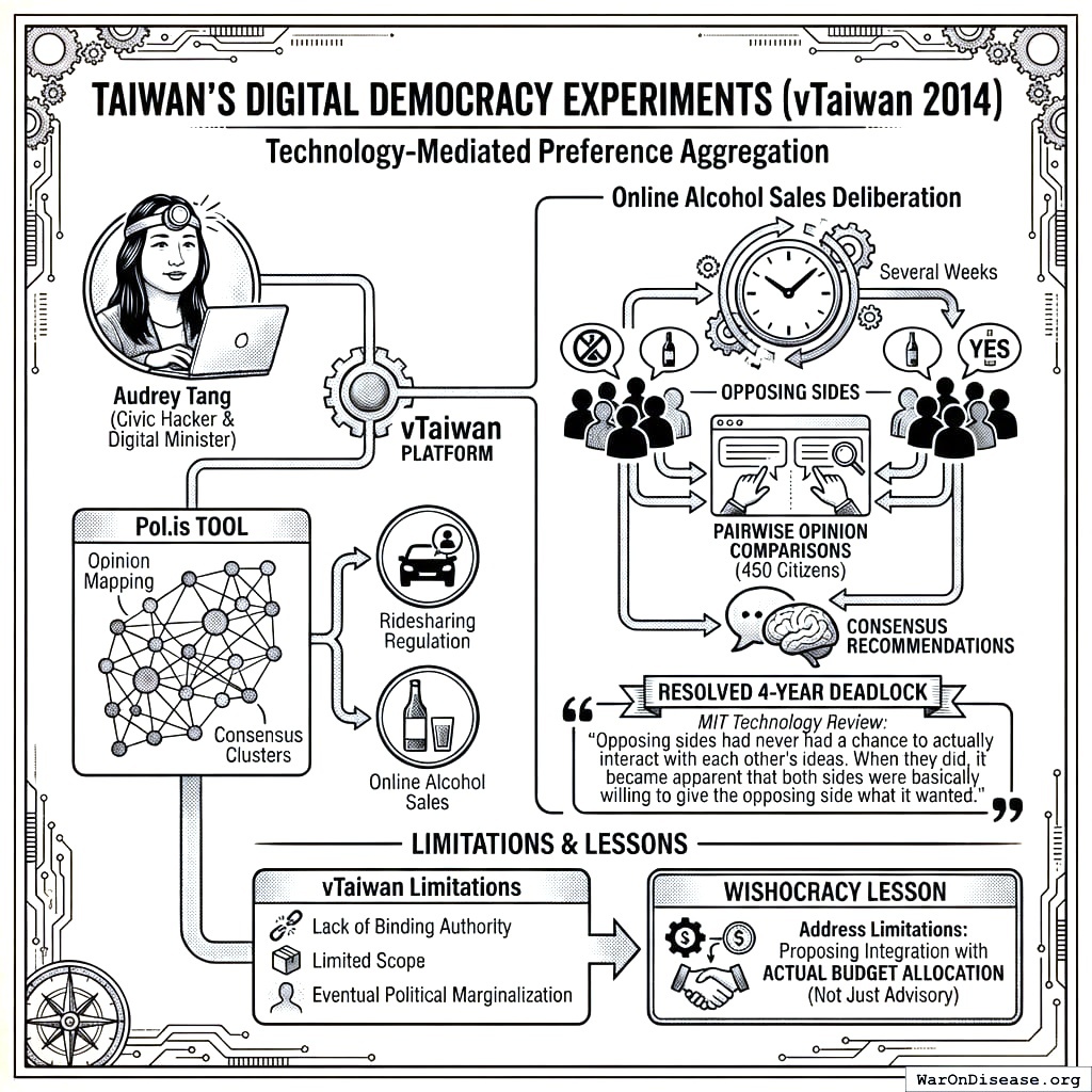
In the alcohol sales deliberation, approximately 450 citizens participated in pairwise opinion comparisons over several weeks, producing consensus recommendations that resolved a four-year regulatory deadlock. The MIT Technology Review noted that ‘opposing sides had never had a chance to actually interact with each other’s ideas. When they did, it became apparent that both sides were basically willing to give the opposing side what it wanted.’
vTaiwan’s limitations (lack of binding authority, limited scope, and eventual political marginalization) provide crucial lessons. Wishocracy addresses these by proposing integration with actual budget allocation rather than advisory recommendations.
5.3 Stanford Participatory Budgeting Platform Research
Academic research on voting interfaces provides direct evidence for RAPPA’s design choices.146 compared cumulative voting, quadratic voting, and traditional ranking methods on Stanford’s Participatory Budgeting platform. Their findings support several Wishocracy design principles.
Voters preferred more expressive methods over simple approval voting, even though expressive methods required more cognitive effort. Participants showed ‘strong intuition for outcomes that provide proportional representation and prioritize fairness.’ The Method of Equal Shares voting rule was perceived as fairer than conventional Greedy allocation.
140 found that voting input formats using rankings or point distribution provided a ‘stronger sense of engagement in the participatory process.’ These findings validate RAPPA’s slider-based allocation over binary choice mechanisms.
5.4 Reference Implementation: Wishocracy.org
To validate the technical feasibility of the RAPPA mechanism, a reference implementation has been deployed at Wishocracy.org. This open-source implementation serves as a pilot environment for:
- Interface Testing: Validating the usability of slider-based pairwise comparisons on mobile and desktop devices.
- Algorithm Verification: Testing the convergence properties of the geometric mean aggregation and eigenvector centrality algorithms under real-world traffic.
- Sybil Resistance: Implementing and stress-testing integration with decentralized identity providers to ensure one-person-one-vote integrity.
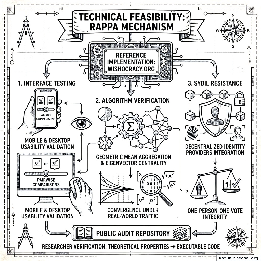
The repository is available for public audit, allowing researchers to verify that the theoretical properties described in Section 3 transform correctly into executable code.
5.4.1 Category Selection and Validation Methodology
The reference implementation uses official federal budget categories drawn from OMB and CBO classifications. Participants see neutral descriptions based on government terminology, not researcher-created labels or value judgments about which programs are “good” or “bad.”
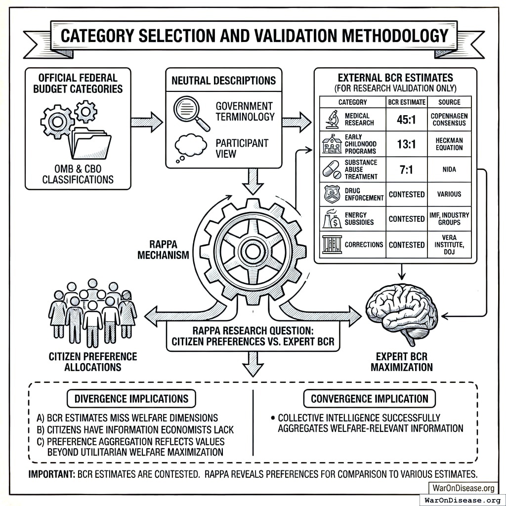
For research validation purposes only (not shown to participants), we track existing benefit-cost ratio estimates from established sources:
| Category | External BCR Estimate | Source |
|---|---|---|
| Medical Research | 45:1 | Copenhagen Consensus |
| Early Childhood Programs | 13:1 | Heckman Equation |
| Substance Abuse Treatment | 7:1 | NIDA |
| Drug Enforcement | Contested | Various |
| Energy Subsidies | Contested | IMF, industry groups |
| Corrections | Contested | Vera Institute, DOJ |
These estimates allow researchers to test a key empirical question: Does RAPPA converge toward allocations that maximize estimated social welfare, or do citizen preferences systematically diverge from expert BCR estimates? Either finding is informative. Convergence suggests collective intelligence successfully aggregates welfare-relevant information. Divergence suggests either (a) BCR estimates miss welfare dimensions citizens care about, (b) citizens have information economists lack, or (c) preference aggregation reflects values beyond utilitarian welfare maximization.
BCR estimates are contested and often politically coded. The same program may have “high ROI” according to one source and “negative ROI” according to another. RAPPA does not assume any particular BCR estimate is correct. The mechanism reveals citizen preferences; researchers can then compare those preferences to various expert estimates.
5.4.2 Zero-Funding Filter Optimization
A naive implementation of RAPPA requires \(\frac{n(n-1)}{2}\) pairwise comparisons for \(n\) categories. For 10 categories, this means 45 pairs per participant (cognitively burdensome and likely to produce survey fatigue).
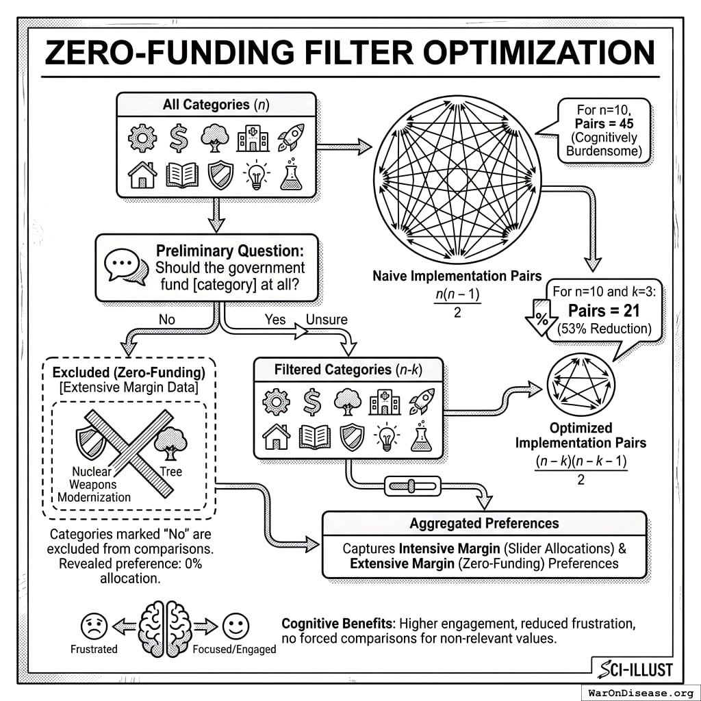
The reference implementation adds a preliminary question: “Should the government fund [category] at all?” Participants can respond Yes, No, or Unsure. Categories marked “No” are excluded from that participant’s pairwise comparisons.
Complexity reduction: If a participant eliminates \(k\) categories, their required comparisons drop from \(\frac{n(n-1)}{2}\) to \(\frac{(n-k)(n-k-1)}{2}\). For \(n=10\) and \(k=3\):
\[ \text{Pairs} = \frac{10 \times 9}{2} = 45 \rightarrow \frac{7 \times 6}{2} = 21 \text{ (53\% reduction)} \]
Information preservation: The zero-funding response is itself preference data. A participant who excludes “Nuclear Weapons Modernization” has revealed an extreme preference (0% allocation) that can be incorporated into the aggregation. The mechanism effectively captures both intensive margin preferences (slider allocations between funded categories) and extensive margin preferences (whether to fund at all).
Cognitive benefits: Participants report higher engagement when they feel the comparisons are relevant to their values. Forcing someone who believes drug enforcement should be defunded to repeatedly compare it against other categories produces frustration without additional information.
5.4.3 Hierarchical Category Structure
A fundamental design question is granularity: should RAPPA operate on a flat list of thousands of budget line items, or on a hierarchical structure that mirrors how budgets are actually organized?
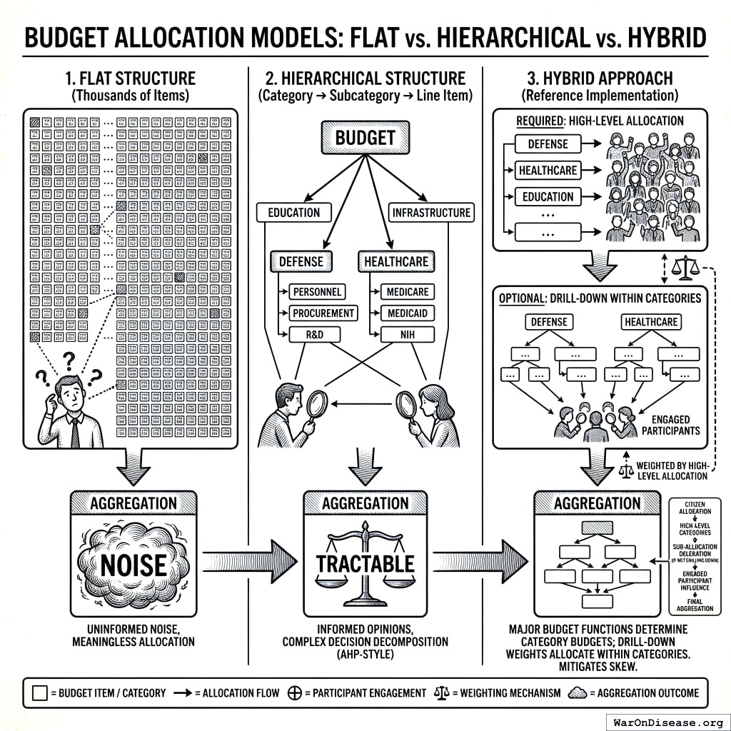
Flat structure (thousands of items, sparse sampling): Each participant sees a random subset of pairs from the full item space. With enough participants, the law of large numbers ensures convergence. However, voters cannot have informed opinions on obscure line items (“Naval Air Systems Command Procurement Account 1319”). Aggregating uninformed noise produces meaningless allocations.
Hierarchical structure (category → subcategory → line item): Participants first allocate across high-level categories (Defense, Healthcare, Education, Infrastructure). Those who want to engage further can drill down: Defense → Personnel vs. Procurement vs. R&D; Healthcare → Medicare vs. Medicaid vs. NIH. This matches how AHP was designed. It decomposes complex decisions into hierarchies of criteria and sub-criteria.
The reference implementation uses a hybrid approach:
- Required: High-level allocation across ~10-15 major budget functions (using OMB classifications)
- Optional: Drill-down within categories of interest
- Aggregation: High-level weights determine category budgets; drill-down weights allocate within categories
This structure has several advantages:
- Citizens can have informed opinions at the category level
- Engaged participants can express fine-grained preferences
- Aggregation is tractable (hierarchical eigenvector methods)
- Results map directly onto existing budget structures
The tradeoff is that participants who don’t drill down delegate sub-allocation to those who do. If only defense hawks drill down within the Defense category, sub-allocations will skew hawkish even if the population-level Defense allocation is modest. Mitigation: weight drill-down responses by high-level allocation (a participant who allocated 5% to Defense gets less influence on Defense sub-allocation than one who allocated 30%).
5.4.4 Framing Bias and Mitigation
How categories are named, described, and presented can systematically bias outcomes. This is not a hypothetical concern. Decades of survey research demonstrate that framing effects routinely shift responses by 10-30 percentage points.
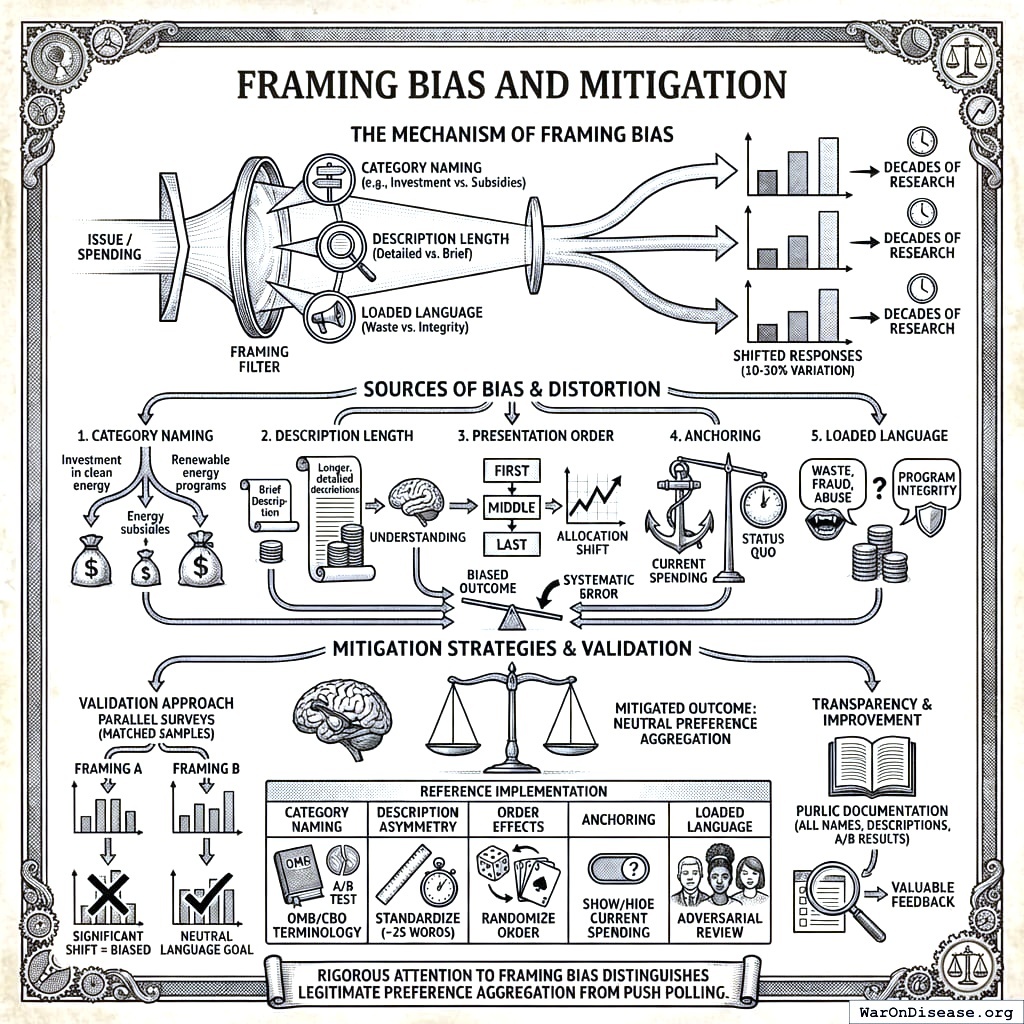
Sources of framing bias:
Category naming: “Investment in clean energy” vs. “Energy subsidies” vs. “Renewable energy programs” will produce different allocations for identical spending.
Description length: Categories with longer, more detailed descriptions may receive more funding simply because participants understand them better.
Presentation order: Categories shown first or last may receive systematically different allocations.
Anchoring: Showing current spending levels may anchor participants toward the status quo.
Loaded language: “Waste, fraud, and abuse” vs. “Program integrity” describes the same spending.
Mitigation strategies in the reference implementation:
| Bias Source | Mitigation |
|---|---|
| Category naming | Use official OMB/CBO terminology; A/B test alternative phrasings |
| Description asymmetry | Standardize descriptions to ~25 words with consistent structure |
| Order effects | Randomize category order for each participant |
| Anchoring | Option to show/hide current spending (test whether it changes allocations) |
| Loaded language | Adversarial review by politically diverse panel before deployment |
Validation approach: Run parallel surveys with different framings on matched samples. If allocations shift significantly based on framing, that framing is biased and should be revised. The goal is descriptions where reasonable people across the political spectrum agree the language is neutral, even if they disagree on the allocation.
Transparency: All category names, descriptions, and any A/B test results should be publicly documented. If critics can identify biased framing, that’s valuable feedback for improvement.
No framing is perfectly neutral. The choice to include or exclude a category is itself a framing decision. But rigorous attention to framing bias distinguishes legitimate preference aggregation from push polling.
6 Addressing Potential Criticisms
6.1 Participation and Digital Divide
Criticism: Digital participation mechanisms exclude citizens without internet access, technological literacy, or time to participate.
Response: Wishocracy should be deployed as a complement to, not replacement for, existing democratic institutions. Multiple access modalities (smartphone apps, web interfaces, public kiosks at libraries and government offices, and paper-based alternatives) can maximize inclusion. Statistical weighting can correct for demographic participation biases, as routinely done in survey research. The cognitive simplicity of pairwise comparisons (unlike lengthy deliberative processes) makes participation accessible to citizens with limited time or formal education.
6.2 Manipulation and Sybil Attacks
Criticism: Bad actors could create multiple accounts or coordinate voting blocs to manipulate outcomes.
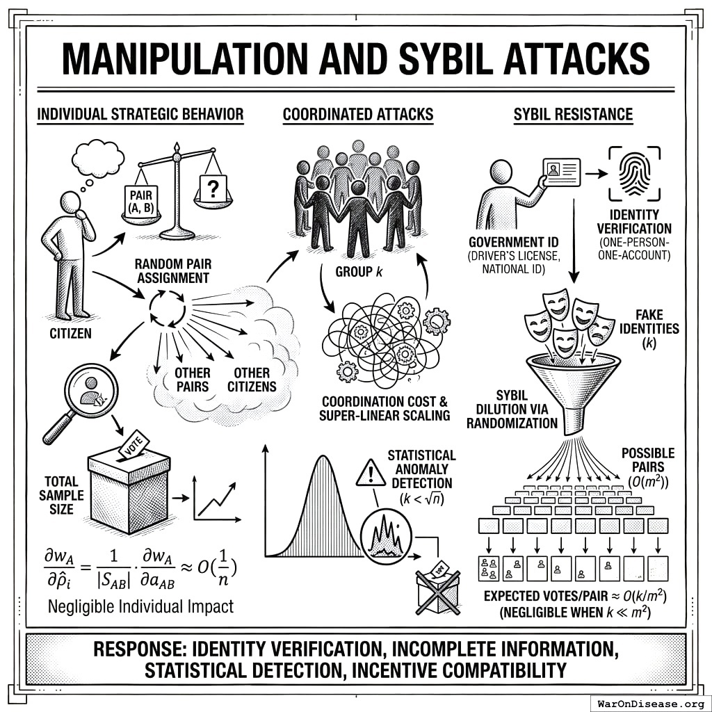
Response: Identity verification through existing government ID systems (driver’s licenses, national ID cards) provides one-person-one-account guarantees. We address manipulation at three levels: individual strategic behavior, coordinated attacks, and formal incentive compatibility.
Individual Strategic Behavior: Consider a citizen evaluating pair \((A, B)\). Under random pair assignment, the citizen does not know: (1) which other pairs they will receive, (2) which pairs other citizens will evaluate, or (3) how others will allocate. This incomplete information structure creates a situation where truthful reporting is a robust heuristic: with random assignment and negligible individual impact, the incentive to game outcomes is weak for most participants. Formally, let \(\rho_i\) be citizen \(i\)’s true valuation ratio and \(\hat{\rho}_i\) be their reported ratio for pair \((A,B)\). The citizen’s influence on the final weight \(w_A\) is:
\[ \frac{\partial w_A}{\partial \hat{\rho}_i} = \frac{1}{|S_{AB}|} \cdot \frac{\partial w_A}{\partial a_{AB}} \]
where \(|S_{AB}|\) is the sample size for pair \((A,B)\). With large \(n\), this influence is negligible (\(O(1/n)\)), making strategic manipulation costly relative to its impact. Moreover, since the citizen cannot predict which of their comparisons will be pivotal, expected utility maximization reduces to truthful reporting across all pairs.
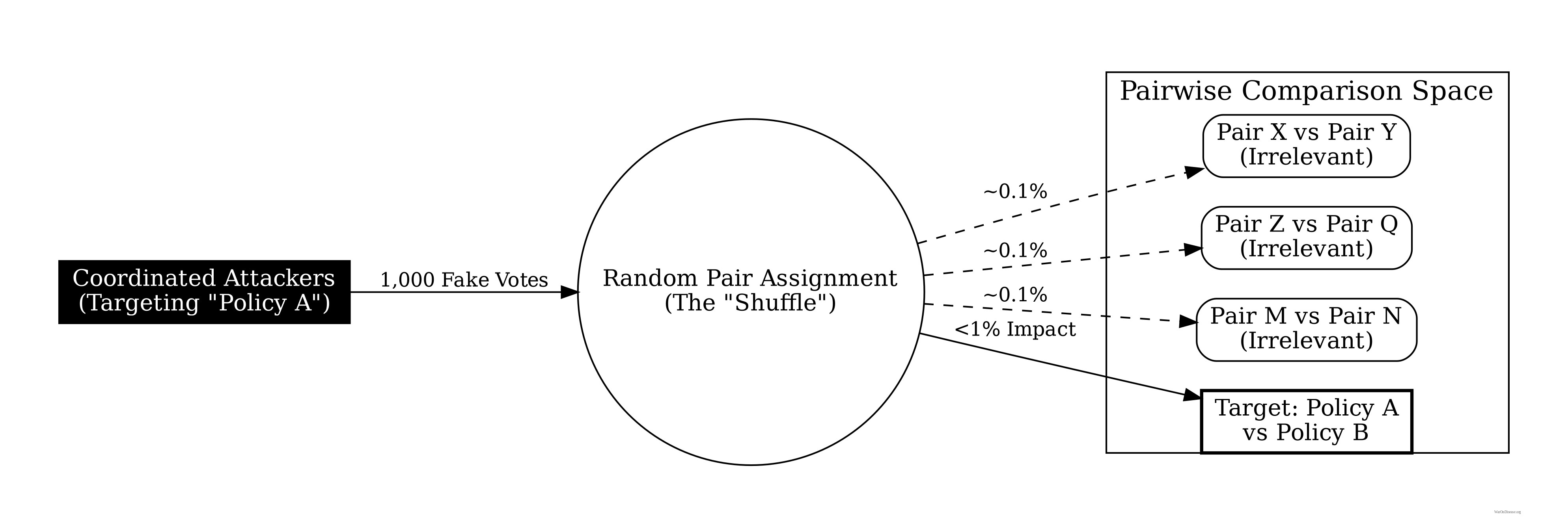
Coordinated Attacks: For a coordinated group of size \(k\) to shift outcome \(A\)’s weight by \(\Delta w\), they must manipulate comparisons involving \(A\) across multiple pairs. With \(m\) outcomes and random assignment, the number of comparisons needed is \(O(m \cdot n / k)\). As \(m\) and \(n\) grow, the coordination cost scales super-linearly while the marginal impact diminishes. Statistical anomaly detection (e.g., comparing individual consistency ratios against population distributions) can identify coordinated patterns with high probability when \(k < \sqrt{n}\).
Sybil Resistance: The incomplete information structure provides inherent Sybil resistance even beyond identity verification. A Sybil attack creating \(k\) fake identities increases the attacker’s allocation power by factor \(k\), but randomization spreads these fake votes across \(O(m^2)\) possible pairs. The expected number of fake votes on any given pair remains \(O(k/m^2)\), which is negligible when \(k \ll m^2\). Combined with identity verification, this makes Sybil attacks both technically difficult and economically irrational.
6.3 Preference Laundering and Manufactured Consent
Criticism: Well-funded interests could use advertising and public relations to shift public preferences before aggregation, laundering elite preferences through ostensibly democratic mechanisms.
Response: This concern applies equally to all democratic mechanisms, including elections. Wishocracy is no more vulnerable to preference manipulation than existing systems and may be more robust due to its continuous, iterative nature. Unlike periodic elections, ongoing preference measurement allows rapid detection of sudden shifts that might indicate manipulation. Transparency requirements for political advertising can be extended to cover preference-shifting campaigns. Ultimately, if citizens’ informed preferences support certain outcomes, those outcomes are legitimate regardless of how preferences formed.
6.4 Complexity of Real Policy Trade-offs
Criticism: Real policy decisions involve complex interdependencies, implementation constraints, and unintended consequences that citizens cannot evaluate.
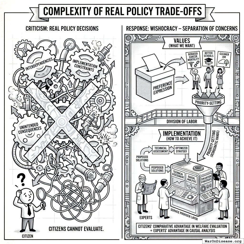
Response: Wishocracy explicitly separates values (what we want) from implementation (how to achieve it). Citizens express preferences over outcomes (reduced cancer mortality, better schools, cleaner air) while experts design and evaluate implementation strategies. The service provider layer allows technical assessment of proposed solutions while keeping priority-setting in democratic hands. This division of labor matches citizens’ comparative advantage in welfare evaluation with experts’ advantage in causal analysis.
6.5 Legitimacy and Accountability
Criticism: Algorithmic aggregation lacks the transparency and accountability of representative institutions.
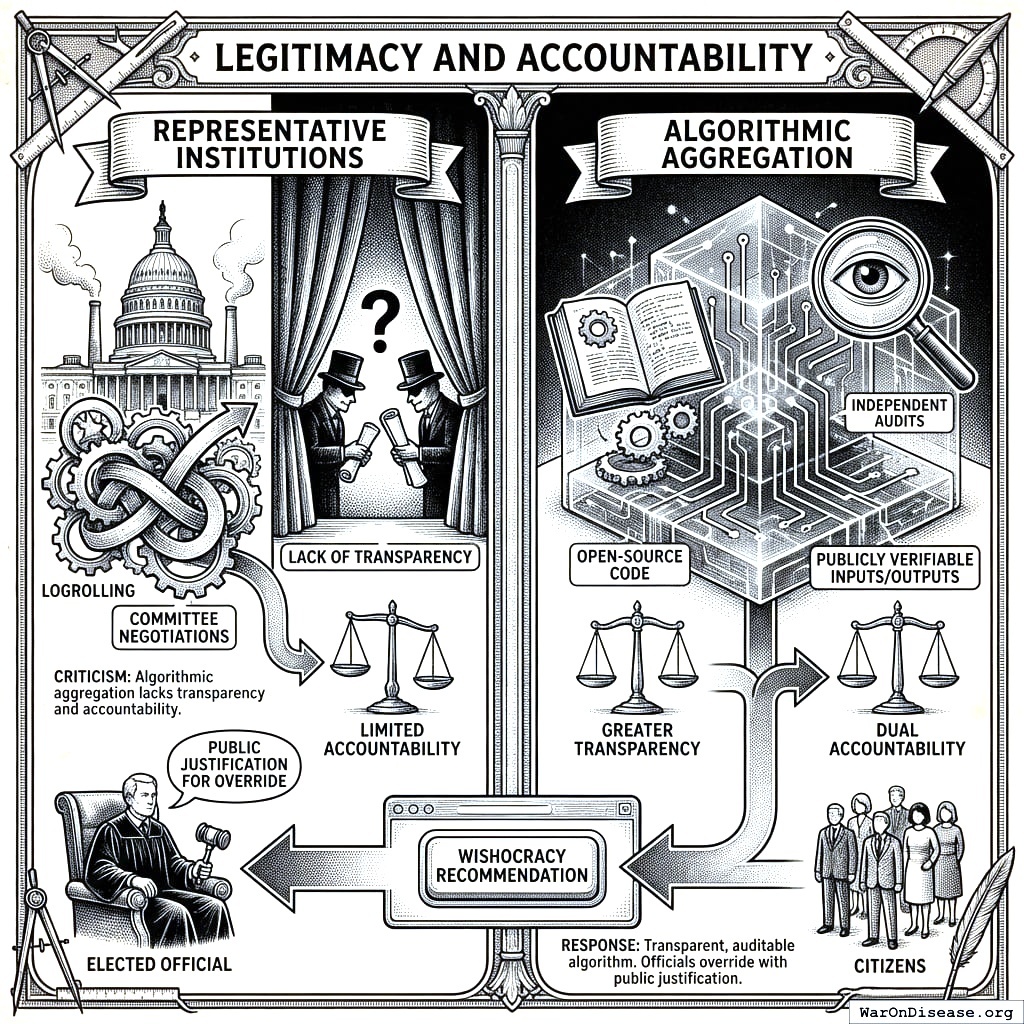
Response: The aggregation algorithm can be made fully transparent and auditable: open-source code, publicly verifiable inputs and outputs, and independent audits. This provides greater transparency than legislative logrolling and committee negotiations. Elected officials retain authority to override Wishocracy recommendations, but must publicly justify departures from expressed citizen preferences. This creates accountability in both directions: citizens to outcomes, and representatives to citizens.
6.6 Failure Modes and Robustness
Low Participation (<1%): When participation falls below critical thresholds, RAPPA faces two degradation modes. First, sampling bias emerges: if only 0.1% of citizens participate and they are systematically unrepresentative (e.g., only highly educated, politically engaged citizens), the aggregated preferences will not reflect population welfare. Second, comparison sparsity increases: with fewer participants, the pairwise comparison matrix becomes increasingly sparse, reducing the reliability of eigenvector estimates.
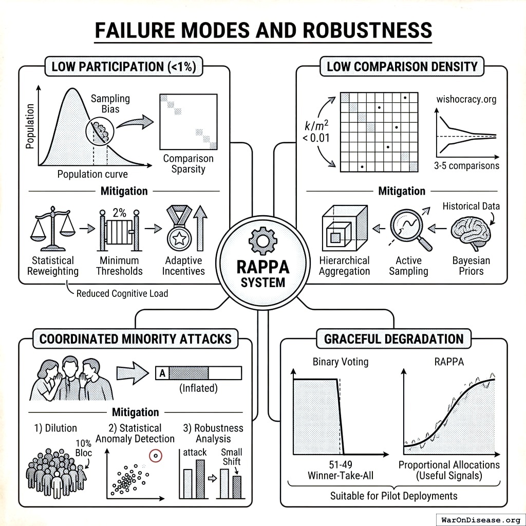
Mitigation: Statistical reweighting can correct for demographic bias, similar to survey research methods. Minimum participation thresholds can be enforced before outcomes become binding: if participation is below (e.g.) 2%, results are treated as advisory rather than binding. Adaptive incentives (entry into lotteries, public recognition) can boost participation. Empirical research suggests that pairwise comparison mechanisms achieve higher engagement than traditional surveys due to reduced cognitive load and increased perceived impact.
Low Comparison Density: As the number of policy priorities \(m\) increases, the required comparisons grow quadratically (\(O(m^2)\)). With fixed participant budgets (each citizen completes \(k\) comparisons), comparison density decreases as \(k/m^2\). At very low densities (\(k/m^2 < 0.01\)), matrix completion methods may produce unstable estimates.
Mitigation: Hierarchical aggregation can reduce effective dimensionality by first aggregating within categories (Healthcare, Education, Defense), then across categories. Active sampling can prioritize comparisons with high uncertainty or inconsistency. Bayesian priors based on expert judgments or historical data can stabilize estimates in sparse regions. Empirical testing at wishocracy.org142 suggests that convergence remains acceptable with as few as 3-5 comparisons per item, meaning systems with 100 priorities can function with ~300-500 comparisons per participant.
Coordinated Minority Attacks: A sophisticated attacker might coordinate a minority bloc to systematically manipulate outcomes. For example, 10% of voters might collude to always allocate 100% to priority \(A\) in any comparison involving \(A\), attempting to artificially inflate \(A\)’s priority weight.
Mitigation: Three defenses address this threat. (1) Dilution: With \(n\) participants and random assignment, the coordinated bloc’s influence on any single comparison is \(O(k/n)\) where \(k\) is bloc size. As shown in Section 5.2, the marginal impact diminishes as \(k/m^2\) when spread across all pairwise comparisons. (2) Statistical anomaly detection: Participants whose allocations are extreme outliers (always 100-0) across many comparisons can be flagged for review. If consistency ratios deviate beyond (e.g.) 3 standard deviations from population mean, weights can be downweighted. (3) Robustness analysis: Final allocations can be recomputed with suspected coordinated voters removed. If outcomes change dramatically (e.g., >20% shift in top priorities), this signals potential manipulation and triggers additional scrutiny.
Graceful Degradation: Critically, RAPPA degrades gracefully rather than catastrophically. Unlike binary voting where a 51-49 split produces winner-take-all outcomes, RAPPA with corrupted or sparse data still produces proportional allocations that approximate true preferences, albeit with increased noise. This property makes RAPPA suitable for pilot deployments where participation may initially be modest: the mechanism provides useful signals even before achieving full-scale adoption.
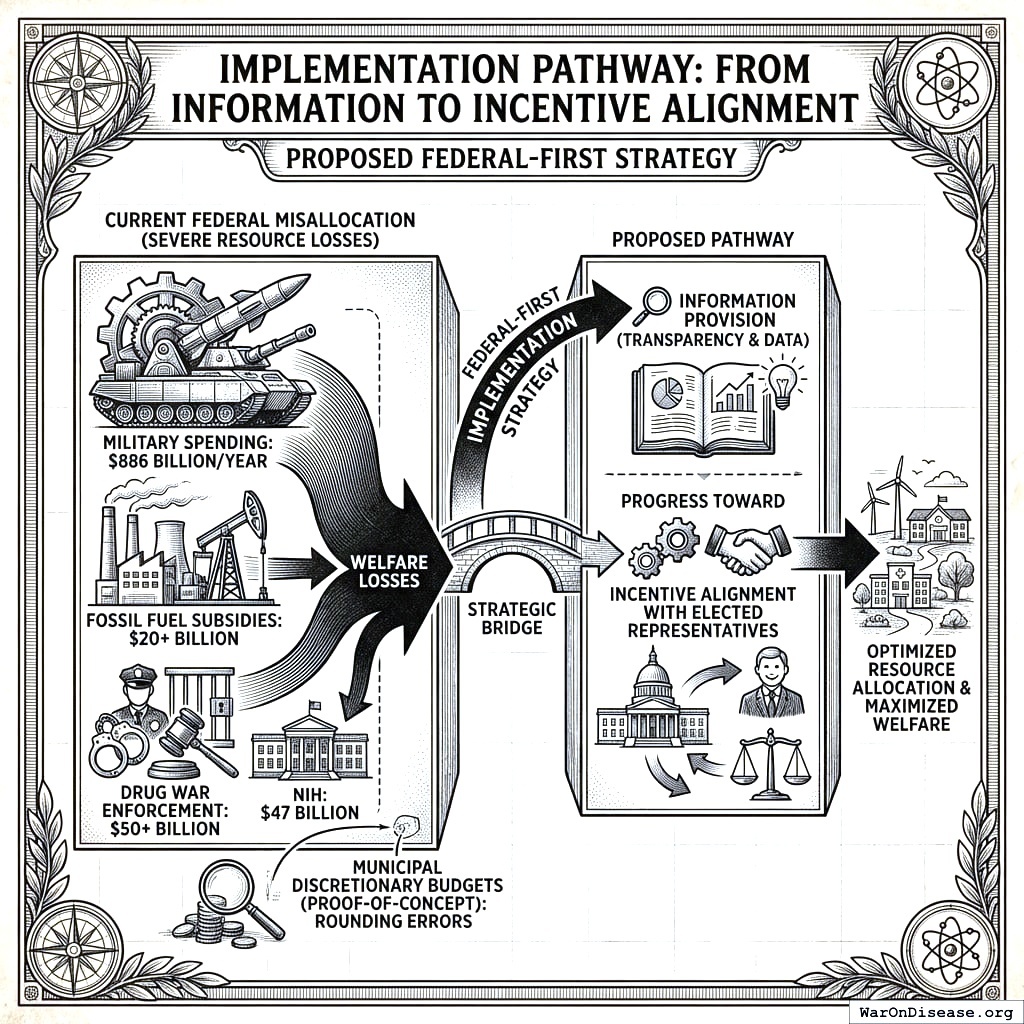
7 Implementation Pathway: From Information to Incentive Alignment
The most severe resource misallocations occur at the federal level: $886 billion annually on military spending versus $47 billion on the NIH, $20+ billion in fossil fuel subsidies, $50+ billion on drug war enforcement. Municipal discretionary budgets, while useful for proof-of-concept, represent rounding errors compared to the welfare losses from federal misallocation. We therefore propose a federal-first implementation strategy that begins with information provision and progresses toward incentive alignment with elected representatives.
7.1 Why Information Alone Fails: Politicians Respond to Incentives
Rankings of government programs by net societal value already exist and are systematically ignored. Rigorous benefit-cost analyses show: pragmatic clinical trials (637:1+ BCR based on RECOVERY trial outcomes147), childhood vaccinations (101:1 BCR), e-government procurement (125:1), maternal health interventions (87:1). These dramatically outperform military spending beyond deterrence requirements (~0.7:1 BCR) and fossil fuel subsidies (negative net societal value). GiveWell, Open Philanthropy, the Copenhagen Consensus, the IMF, and numerous academic institutions produce similar analyses.
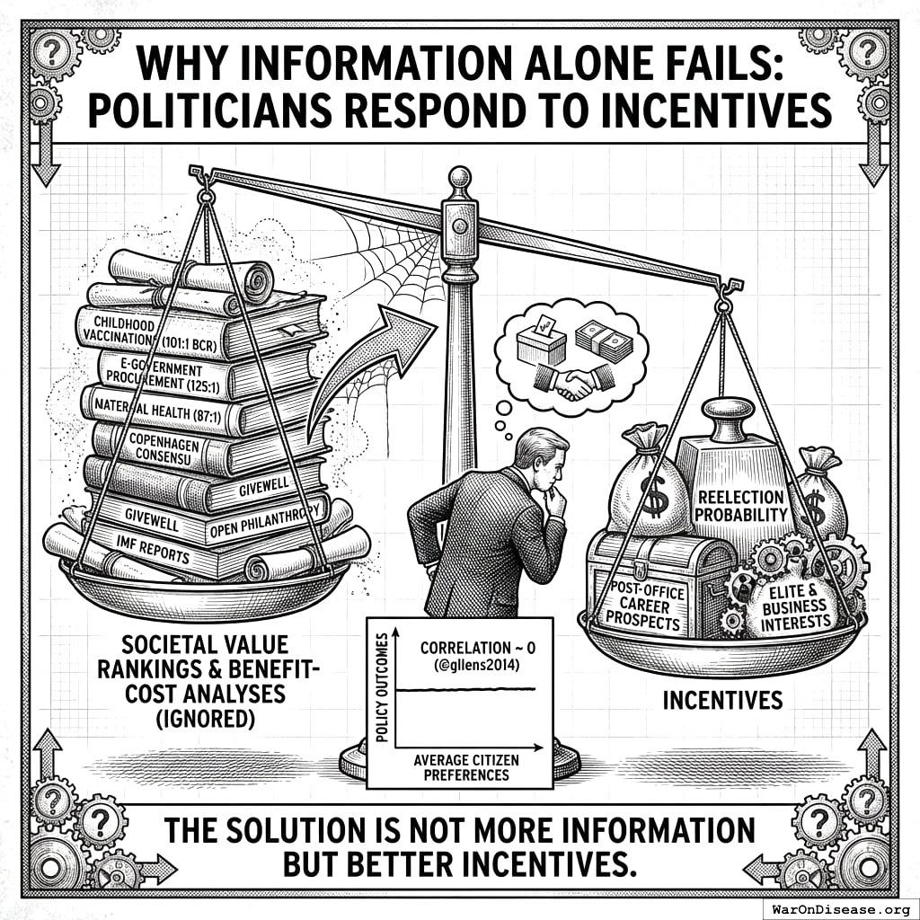
Yet government spending patterns have not shifted.143 analyzed 1,779 policy decisions and found that “economic elites and organized groups representing business interests have substantial independent impacts on U.S. government policy, while mass-based interest groups and average citizens have little or no independent influence.” The correlation between average citizen preferences and policy outcomes was effectively zero.
The marginal value of producing another ranking is zero. Politicians already know which programs produce net societal value. They don’t act on this knowledge because acting on it doesn’t appear in their utility function (reelection probability, campaign contributions, post-office career prospects). The solution is not more information but better incentives.
7.2 Three-Phase Implementation
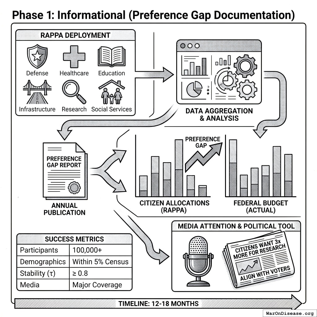
7.2.1 Phase 1: Informational (Preference Gap Documentation)
Objective: Establish RAPPA as a credible measure of citizen preferences and document the gap between public preferences and actual federal allocations.
Mechanism:
- Deploy RAPPA on major federal budget categories (Defense, Healthcare, Education, Infrastructure, Research, Social Services, etc.)
- Aggregate preferences from a statistically representative sample of U.S. adults
- Publish annual “Preference Gap Report” showing divergence between RAPPA allocations and actual federal budget
- Generate media attention around largest divergences (e.g., “Citizens would allocate 3x more to medical research and 40% less to military”)
Success Metrics:
| Metric | Target |
|---|---|
| Participants | 100,000+ annually |
| Demographic representativeness | Within 5% of census on key demographics |
| Preference stability (year-over-year) | τ ≥ 0.8 |
| Media coverage | Major outlet coverage of Preference Gap Report |
Timeline: 12-18 months to establish credibility and baseline measurements.
Why this works: Information alone won’t change policy, but it creates the foundation for Phase 2. The Preference Gap Report becomes a political tool: candidates can campaign on “aligning with citizen preferences” and opponents can be attacked for “ignoring what voters actually want.”
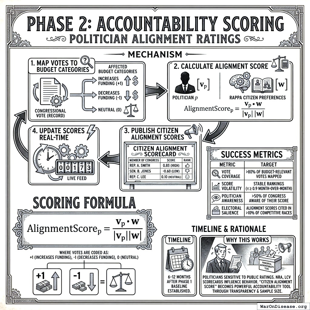
7.2.2 Phase 2: Accountability Scoring (Politician Alignment Ratings)
Objective: Create a public scoring system that rates elected officials based on how their voting records correlate with RAPPA-expressed citizen preferences.
Mechanism:
- Map each congressional vote to affected budget categories
- Calculate alignment score: correlation between politician’s voting pattern and RAPPA preference weights
- Publish “Citizen Alignment Scores” for all members of Congress
- Update scores in real-time as new votes occur
Scoring Formula:
For politician \(p\) with voting record \(\mathbf{v}_p\) across \(k\) budget-relevant votes, and RAPPA preference vector \(\mathbf{w}\):
\[ \text{AlignmentScore}_p = \frac{\mathbf{v}_p \cdot \mathbf{w}}{|\mathbf{v}_p||\mathbf{w}|} \]
where votes are coded as +1 (increases funding for category), -1 (decreases funding), or 0 (neutral).
Success Metrics:
| Metric | Target |
|---|---|
| Vote coverage | >80% of budget-relevant votes mapped |
| Score volatility | Stable rankings (τ ≥ 0.9 month-over-month) |
| Politician awareness | >50% of Congress aware of their score |
| Electoral salience | Alignment scores cited in >10% of competitive races |
Timeline: 6-12 months after Phase 1 baseline established.
Why this works: Politicians are highly sensitive to public ratings. The NRA’s letter grades, the League of Conservation Voters’ scorecard, and similar systems demonstrably influence politician behavior. A “Citizen Alignment Score” backed by transparent methodology and large sample sizes becomes a powerful accountability tool.
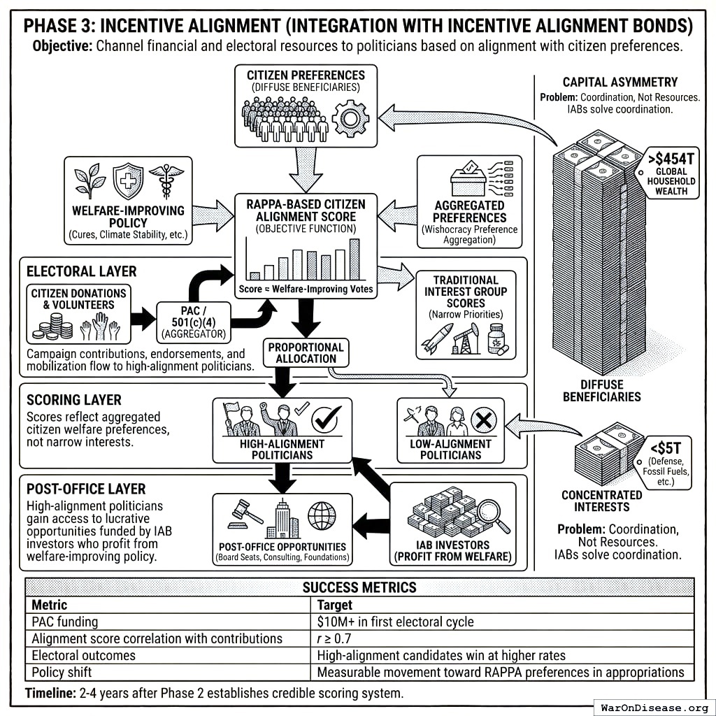
7.2.3 Phase 3: Incentive Alignment (Integration with Incentive Alignment Bonds)
Objective: Channel financial and electoral resources to politicians based on their alignment with citizen preferences, making welfare-improving votes incentive-compatible.
Mechanism:
Wishocracy’s preference aggregation integrates with Incentive Alignment Bonds (IABs), a mechanism design approach to political economy. IABs create three layers of incentive alignment:
Electoral Layer: Campaign contributions, endorsements, and volunteer mobilization flow to high-alignment politicians. A PAC or 501(c)(4) aggregates small-dollar donations from citizens and allocates them proportionally to Citizen Alignment Scores.
Scoring Layer: The RAPPA-based Citizen Alignment Score provides the objective function that IABs optimize. Unlike traditional interest group scores (which reflect narrow priorities), RAPPA scores reflect aggregated citizen welfare preferences.
Post-Office Layer: High-alignment politicians gain access to lucrative post-office opportunities (board seats, consulting, foundation positions) funded by IAB investors who profit from welfare-improving policy adoption.
Politicians currently face incentives that reward serving concentrated interests (weapons manufacturers, pharmaceutical incumbents, fossil fuel producers) at the expense of diffuse beneficiaries (citizens who would benefit from cures, climate stability, reduced existential risk). IABs flip this calculus by making the diffuse beneficiaries’ preferences financially consequential.
Capital Asymmetry: Diffuse beneficiaries collectively control far more capital than concentrated interests. Global household wealth exceeds $454T; the combined market capitalization of industries benefiting from misallocation (weapons manufacturers, fossil fuels, etc.) is under $5T. The problem is coordination, not resources. IABs solve the coordination problem by creating a vehicle for diffuse beneficiaries to pool resources and direct them toward aligned politicians.
Success Metrics:
| Metric | Target |
|---|---|
| PAC funding | $10M+ in first electoral cycle |
| Alignment score correlation with contributions | r ≥ 0.7 |
| Electoral outcomes | High-alignment candidates win at higher rates than low-alignment |
| Policy shift | Measurable movement toward RAPPA preferences in appropriations |
Timeline: 2-4 years after Phase 2 establishes credible scoring system.
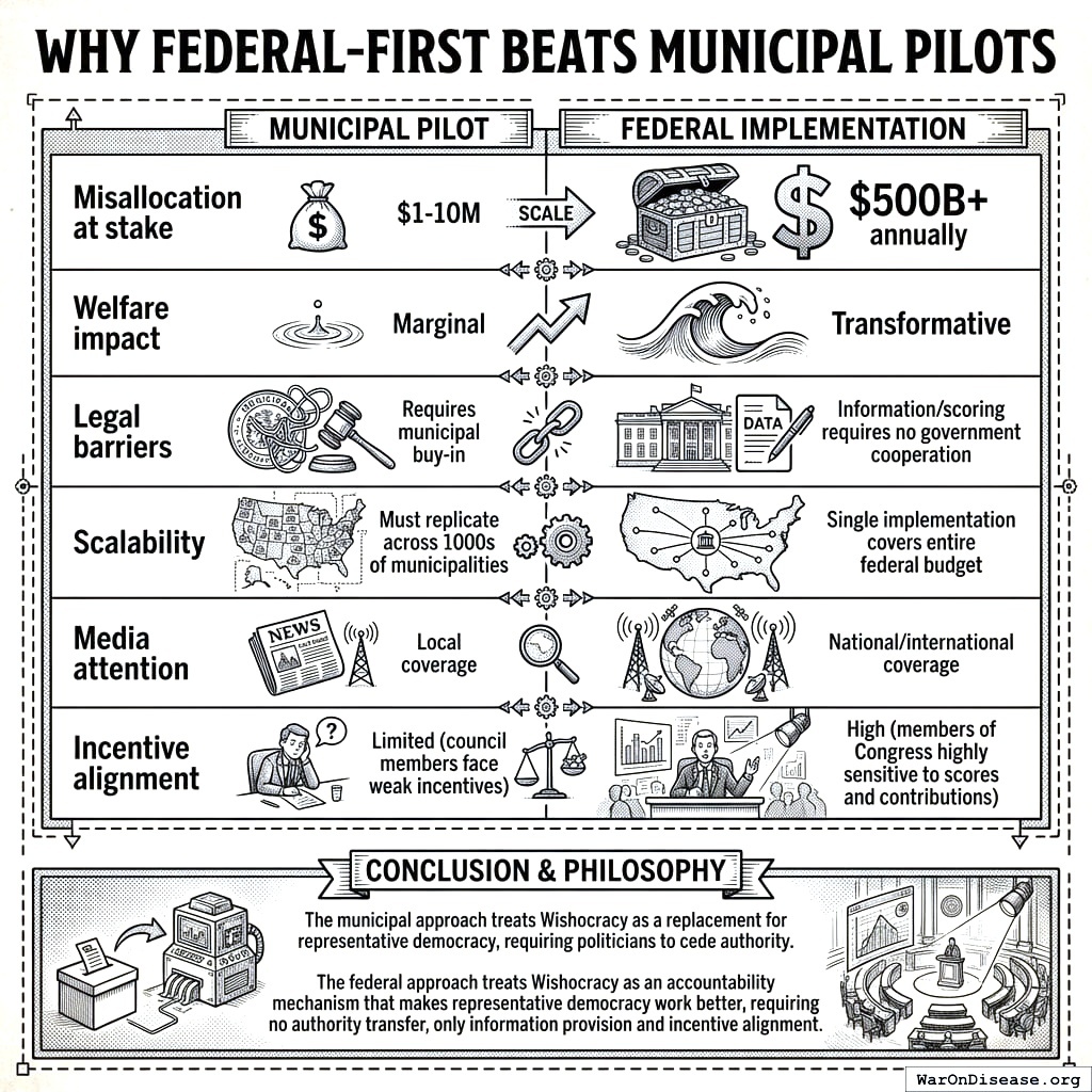
7.3 Why Federal-Scale Priorities
Municipal participatory budgeting has achieved real successes. Porto Alegre’s experience demonstrates that citizen participation can improve service delivery. However, RAPPA addresses a different challenge than traditional participatory budgeting.
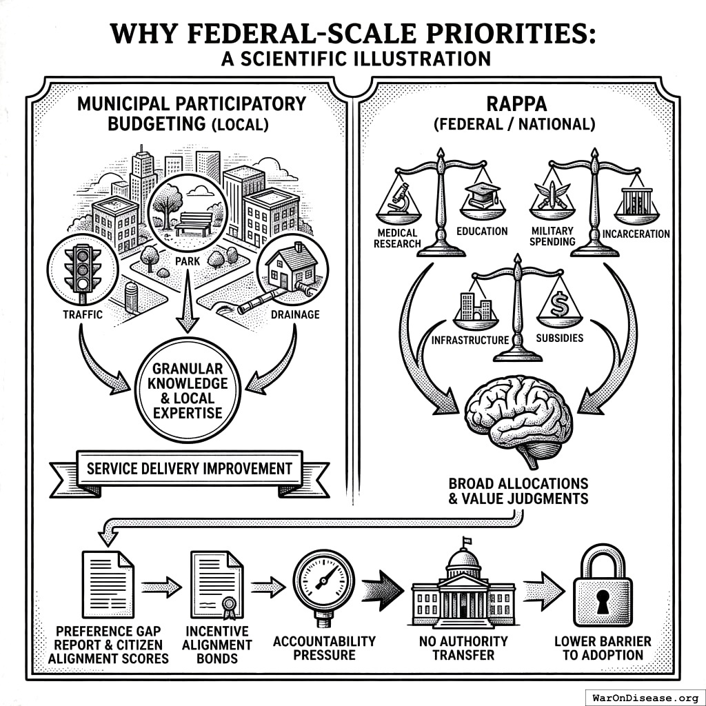
Local budget decisions often require granular knowledge: which intersection needs a traffic light, which park needs renovation, which neighborhood lacks adequate drainage. These decisions benefit from local expertise and community-specific information that outsiders lack.
National budget priorities operate differently. Citizens have strong preferences about broad allocations: medical research versus military spending, education versus incarceration, infrastructure versus subsidies. They can make these judgments without needing neighborhood-level expertise. These are value judgments about societal priorities, not technical assessments of local conditions.
RAPPA is designed for the latter: large option spaces where citizens hold meaningful preferences but lack any tractable mechanism to express them across all dimensions simultaneously. The federal budget, with its trillion-dollar misallocations between citizen preferences and actual spending, represents the highest-leverage application.
Additionally, the federal approach requires no authority transfer. Publishing a “Preference Gap Report” and Citizen Alignment Scores is pure information provision. Combined with Incentive Alignment Bonds, this creates accountability pressure without asking any politician to cede decision-making authority. This is a significantly lower barrier to adoption than municipal pilots that require city councils to delegate budget control.
7.4 Evaluation Framework
Despite the federal focus, rigorous evaluation remains essential:
7.4.1 Preference Aggregation Quality
| Metric | Measurement | Success Threshold |
|---|---|---|
| Test-retest reliability | Correlation on repeated pairs | r ≥ 0.7 |
| Aggregate stability | Year-over-year rank correlation | τ ≥ 0.8 |
| Demographic representativeness | Comparison to census | No significant difference |
| Manipulation resistance | Robustness to outlier removal | <5% shift in top priorities |
7.4.2 Accountability System Effectiveness
| Metric | Measurement | Success Threshold |
|---|---|---|
| Score predictive validity | Correlation between alignment score and future votes | r ≥ 0.6 |
| Electoral salience | Candidates referencing alignment scores | >10% of competitive races |
| Behavioral response | Politicians shifting votes after score publication | Measurable movement |
7.4.3 Incentive Alignment Impact
| Metric | Measurement | Success Threshold |
|---|---|---|
| Contribution-alignment correlation | PAC dollars vs. alignment score | r ≥ 0.7 |
| Electoral outcomes | Win rate by alignment quintile | Positive gradient |
| Policy outcomes | Appropriations shift toward RAPPA preferences | Measurable movement |
| Preference gap reduction | Year-over-year change in divergence | Decreasing trend |
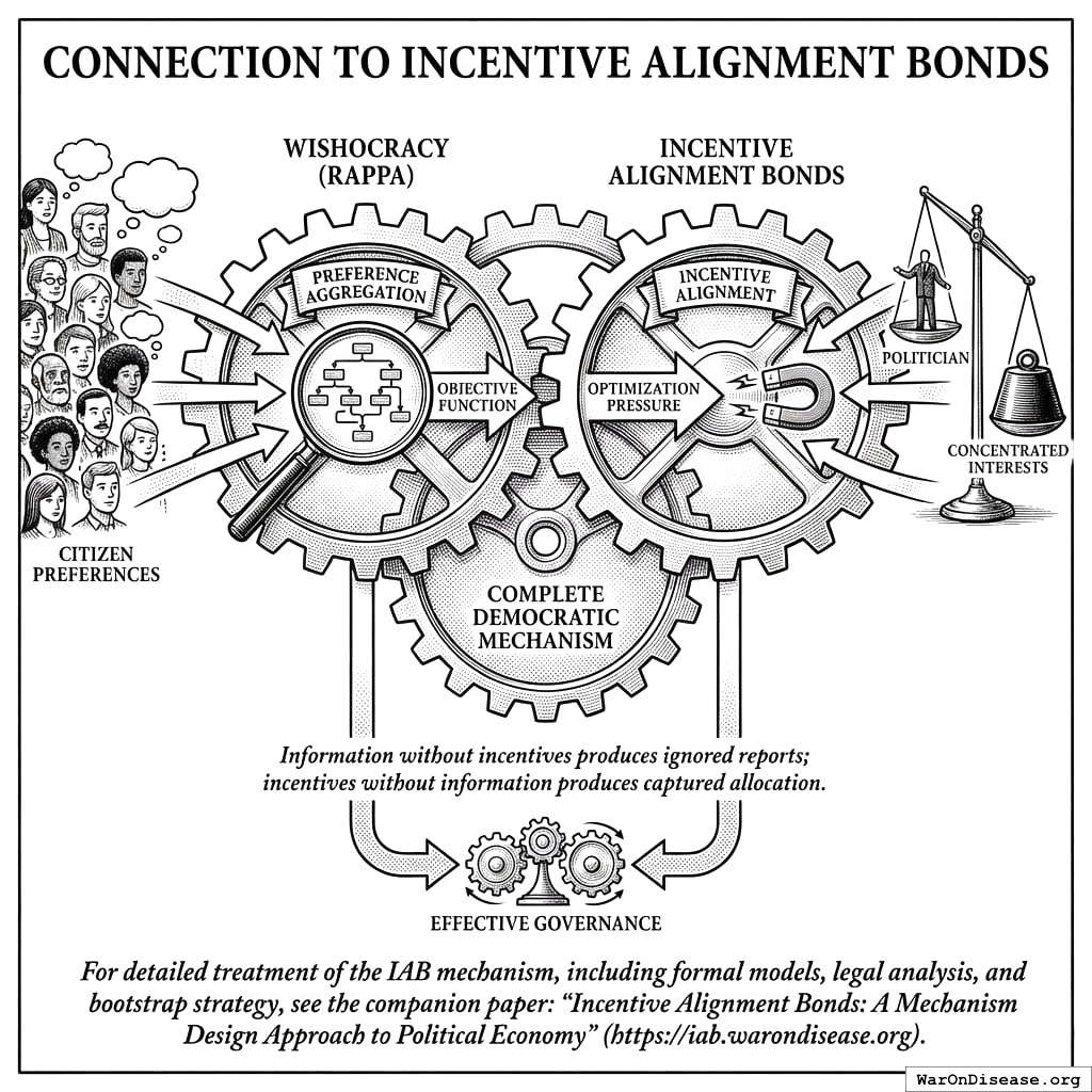
7.5 Connection to Incentive Alignment Bonds
Wishocracy and Incentive Alignment Bonds are complementary mechanisms addressing different parts of the democratic failure:
Wishocracy (RAPPA) solves the preference aggregation problem: How do we know what citizens actually want across complex, multidimensional policy spaces?
Incentive Alignment Bonds solve the incentive alignment problem: How do we make politicians act on citizen preferences rather than concentrated interests?
Together, they form a complete system: RAPPA provides the objective function (what to optimize for), and IABs provide the optimization pressure (why politicians should care). Neither mechanism alone is sufficient: information without incentives produces ignored reports; incentives without information produces captured allocation.
For detailed treatment of the IAB mechanism, including formal models, legal analysis, and bootstrap strategy, see the companion paper: Incentive Alignment Bonds: A Mechanism Design Approach to Political Economy.
7.6 Connection to Optimocracy
Wishocracy and Optimocracy represent two distinct approaches to governance reform that can function independently or in combination:
- Wishocracy is democratic: citizens express preferences, and the mechanism aggregates them. The output is a preference signal that politicians can choose to follow or ignore (absent incentive mechanisms).
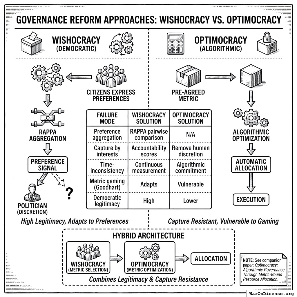
- Optimocracy is algorithmic: a pre-agreed metric is optimized automatically, with minimal political discretion. The output is an allocation that executes regardless of political preferences.
These approaches address different failure modes:
| Failure Mode | Wishocracy Solution | Optimocracy Solution |
|---|---|---|
| Preference aggregation | RAPPA pairwise comparison | N/A (metric pre-selected) |
| Capture by interests | Accountability scores | Remove political discretion |
| Time-inconsistency | Continuous measurement | Algorithmic commitment |
| Metric gaming (Goodhart) | Adapts to changing preferences | Vulnerable |
| Democratic legitimacy | High (citizen input) | Lower (algorithm decides) |
A hybrid architecture might use Wishocracy for metric selection (citizens choose what to optimize) and Optimocracy for metric optimization (algorithms allocate to maximize the chosen metric). This combines democratic legitimacy at the constitutional level with capture resistance at the execution level.
For detailed treatment of algorithmic governance, including smart contract specifications and oracle design, see the companion paper: Optimocracy: Algorithmic Governance Through Outcome-Optimizing Resource Allocation.
8 Conclusion
Representative democracy’s principal-agent problem is not a bug but a structural feature: elected officials inevitably face incentives that diverge from citizen welfare. No amount of campaign finance reform, term limits, or transparency requirements can eliminate the fundamental misalignment between representatives who must satisfy donors and constituents simultaneously. Meanwhile, direct democracy mechanisms remain cognitively infeasible for the complex, multidimensional trade-offs that characterize modern governance.
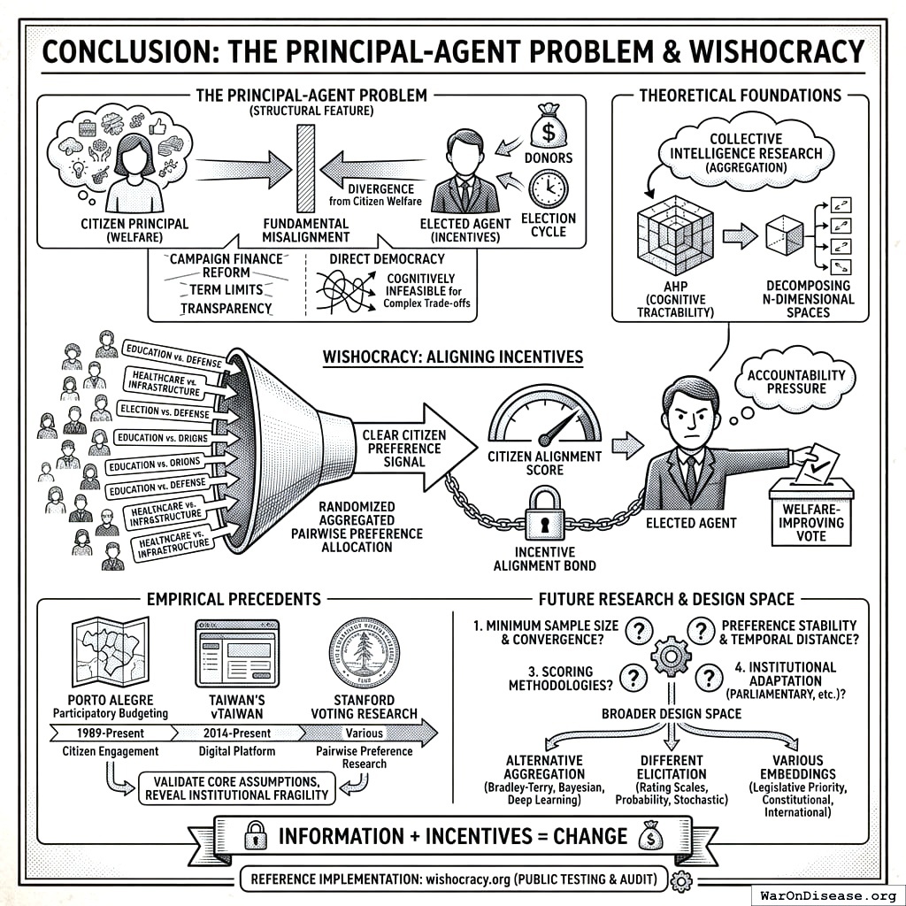
Wishocracy offers a different approach: rather than replacing representatives, align their incentives with citizen preferences. Through Randomized Aggregated Pairwise Preference Allocation, the mechanism aggregates citizen preferences into a clear signal of what voters actually want. Combined with Citizen Alignment Scores and Incentive Alignment Bonds, this creates accountability pressure that makes welfare-improving votes politically and financially rewarding. The theoretical foundations combine the Analytic Hierarchy Process (for cognitive tractability) with collective intelligence research (for aggregation), decomposing n-dimensional preference spaces into simple pairwise comparisons that any citizen can complete.
The empirical precedents from Porto Alegre’s participatory budgeting, Taiwan’s vTaiwan platform, and Stanford’s voting research demonstrate that citizens can and will engage productively with pairwise preference-expressing mechanisms. These real-world experiments validate the core assumptions underlying Wishocracy while revealing the institutional fragility of advisory mechanisms that lack connection to electoral incentives.
Several questions require further research. First, what is the minimum sample size and comparison density needed for preference convergence across different problem domains? Second, how does preference stability vary with issue complexity and temporal distance? Third, what scoring methodologies best capture alignment between voting records and citizen preferences? Fourth, how can the mechanism be adapted for parliamentary systems, multi-party democracies, and other institutional contexts beyond the U.S. Congress?
The mechanism design presented here represents one point in a broader design space of democratic innovations. Alternative aggregation methods (Bradley-Terry models, Bayesian updating, deep learning approaches), different elicitation formats (rating scales, probability distributions, stochastic choice), and various institutional embeddings (legislative priority-setting, constitutional conventions, international treaty negotiations) warrant systematic exploration.
Wishocracy addresses the central failure mode of democratic governance: the principal-agent problem that corrupts representative institutions. The mechanism combines four elements: AHP’s cognitive tractability, slider-based preference intensity capture, collective intelligence aggregation, and (critically) integration with incentive mechanisms that make representatives care about alignment scores. Information alone changes nothing. Information plus incentives can change everything.
The mechanism is implementable with current technology, grounded in validated theory, and supported by empirical precedents. A reference implementation is available at wishocracy.org for public testing and audit. Whether Wishocracy can achieve its theoretical promise (truly aligning public resource allocation with citizen welfare) remains an open empirical question that only real-world deployment can answer.
9 Appendix A: The Service Provider Layer
Important: Service providers represent a distinct, separate layer from the core RAPPA mechanism. While RAPPA handles democratic preference aggregation to determine what society should prioritize, service providers address the orthogonal question of how to achieve those priorities.
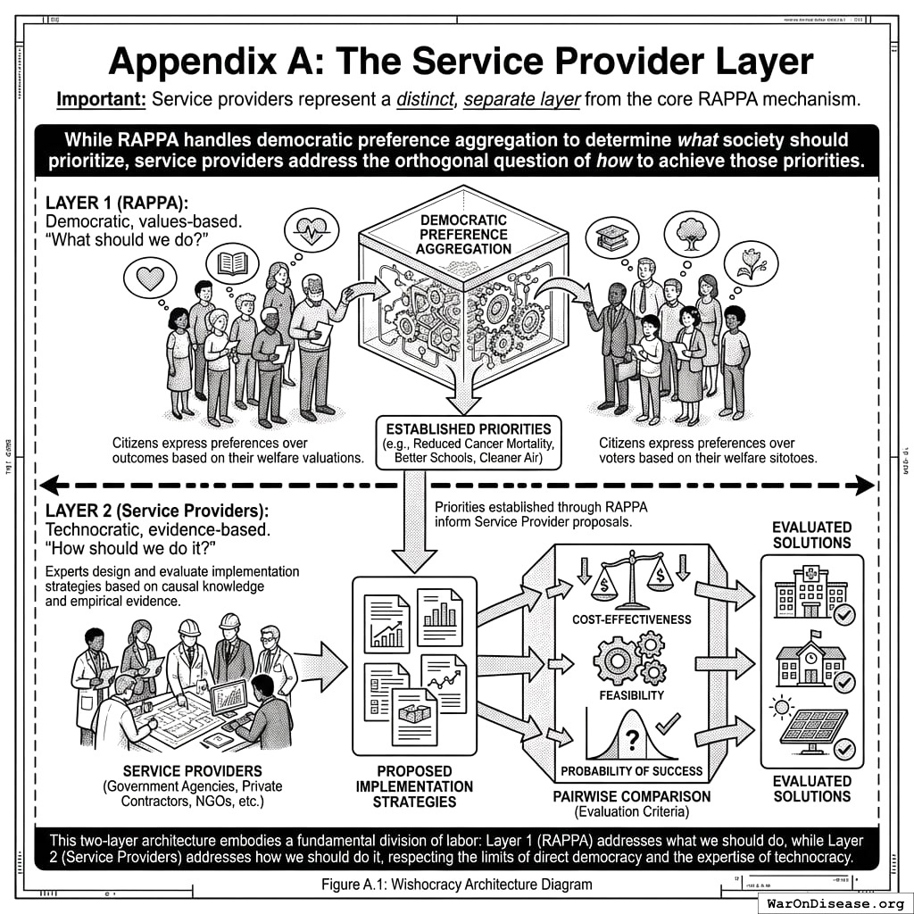
Once priorities are established through RAPPA, Wishocracy introduces this second layer for solution generation and evaluation. Service providers (which may include government agencies, private contractors, NGOs, or other qualified entities) form around specific priorities to propose implementation strategies. These proposals are subject to pairwise comparison using different evaluation criteria: cost-effectiveness, feasibility, and probability of success.
This two-layer architecture embodies a fundamental division of labor:
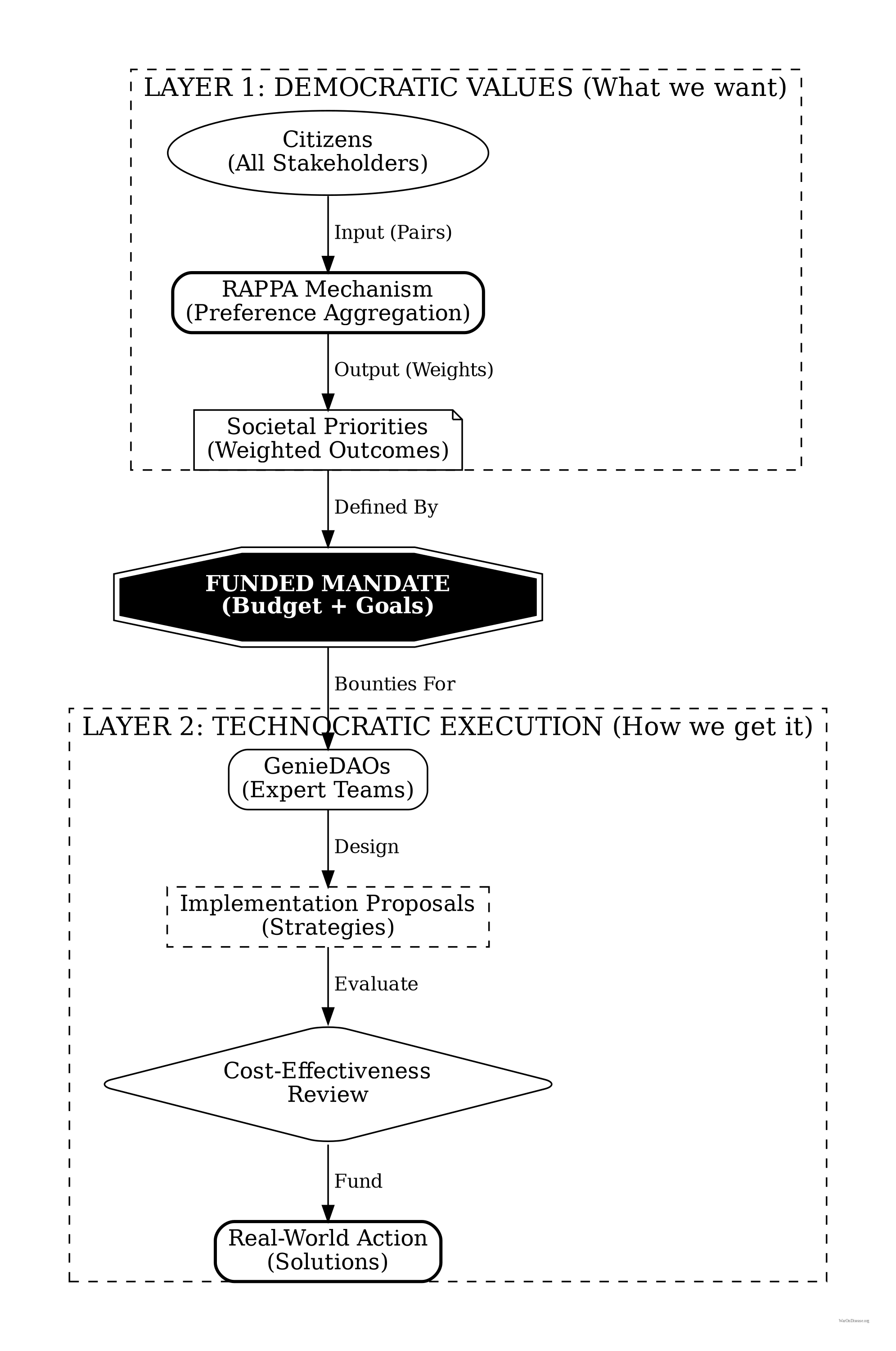
Layer 1 (RAPPA): Democratic, values-based. “What should we do?” Citizens express preferences over outcomes (reduced cancer mortality, better schools, cleaner air) based on their welfare valuations.
Layer 2 (Service Providers): Technocratic, evidence-based. “How should we do it?” Experts design and evaluate implementation strategies based on causal knowledge and empirical evidence.
This separation addresses a key criticism of technocracy (experts shouldn’t determine societal values) while respecting the limits of direct democracy (citizens cannot evaluate complex implementation trade-offs). Each layer operates where its participants have comparative advantage: citizens in welfare evaluation, experts in causal analysis.
References
1.
NIH Common Fund. NIH pragmatic trials: Minimal funding despite 30x cost advantage. NIH Common Fund: HCS Research Collaboratory https://commonfund.nih.gov/hcscollaboratory (2025)
The NIH Pragmatic Trials Collaboratory funds trials at $500K for planning phase, $1M/year for implementation-a tiny fraction of NIH’s budget. The ADAPTABLE trial cost $14 million for 15,076 patients (= $929/patient) versus $420 million for a similar traditional RCT (30x cheaper), yet pragmatic trials remain severely underfunded. PCORnet infrastructure enables real-world trials embedded in healthcare systems, but receives minimal support compared to basic research funding. Additional sources: https://commonfund.nih.gov/hcscollaboratory | https://pcornet.org/wp-content/uploads/2025/08/ADAPTABLE_Lay_Summary_21JUL2025.pdf | https://www.ncbi.nlm.nih.gov/pmc/articles/PMC5604499/
.2.
NIH. Antidepressant clinical trial exclusion rates. Zimmerman et al. https://pubmed.ncbi.nlm.nih.gov/26276679/ (2015)
Mean exclusion rate: 86.1% across 158 antidepressant efficacy trials (range: 44.4% to 99.8%) More than 82% of real-world depression patients would be ineligible for antidepressant registration trials Exclusion rates increased over time: 91.4% (2010-2014) vs. 83.8% (1995-2009) Most common exclusions: comorbid psychiatric disorders, age restrictions, insufficient depression severity, medical conditions Emergency psychiatry patients: only 3.3% eligible (96.7% excluded) when applying 9 common exclusion criteria Only a minority of depressed patients seen in clinical practice are likely to be eligible for most AETs Note: Generalizability of antidepressant trials has decreased over time, with increasingly stringent exclusion criteria eliminating patients who would actually use the drugs in clinical practice Additional sources: https://pubmed.ncbi.nlm.nih.gov/26276679/ | https://pubmed.ncbi.nlm.nih.gov/26164052/ | https://www.wolterskluwer.com/en/news/antidepressant-trials-exclude-most-real-world-patients-with-depression
.3.
CNBC. Warren buffett’s career average investment return. CNBC https://www.cnbc.com/2025/05/05/warren-buffetts-return-tally-after-60-years-5502284percent.html (2025)
Berkshire’s compounded annual return from 1965 through 2024 was 19.9%, nearly double the 10.4% recorded by the S&P 500. Berkshire shares skyrocketed 5,502,284% compared to the S&P 500’s 39,054% rise during that period. Additional sources: https://www.cnbc.com/2025/05/05/warren-buffetts-return-tally-after-60-years-5502284percent.html | https://www.slickcharts.com/berkshire-hathaway/returns
.4.
World Health Organization. WHO global health estimates 2024. World Health Organization https://www.who.int/data/gho/data/themes/mortality-and-global-health-estimates (2024)
Comprehensive mortality and morbidity data by cause, age, sex, country, and year Global mortality: 55-60 million deaths annually Lives saved by modern medicine (vaccines, cardiovascular drugs, oncology): 12M annually (conservative aggregate) Leading causes of death: Cardiovascular disease (17.9M), Cancer (10.3M), Respiratory disease (4.0M) Note: Baseline data for regulatory mortality analysis. Conservative estimate of pharmaceutical impact based on WHO immunization data (4.5M/year from vaccines) + cardiovascular interventions (3.3M/year) + oncology (1.5M/year) + other therapies. Additional sources: https://www.who.int/data/gho/data/themes/mortality-and-global-health-estimates
.5.
GiveWell. GiveWell cost per life saved for top charities (2024). GiveWell: Top Charities https://www.givewell.org/charities/top-charities
General range: $3,000-$5,500 per life saved (GiveWell top charities) Helen Keller International (Vitamin A): $3,500 average (2022-2024); varies $1,000-$8,500 by country Against Malaria Foundation: $5,500 per life saved New Incentives (vaccination incentives): $4,500 per life saved Malaria Consortium (seasonal malaria chemoprevention): $3,500 per life saved VAS program details: $2 to provide vitamin A supplements to child for one year Note: Figures accurate for 2024. Helen Keller VAS program has wide country variation ($1K-$8.5K) but $3,500 is accurate average. Among most cost-effective interventions globally Additional sources: https://www.givewell.org/charities/top-charities | https://www.givewell.org/charities/helen-keller-international | https://ourworldindata.org/cost-effectiveness
.6.
AARP. Unpaid caregiver hours and economic value. AARP 2023 https://www.aarp.org/caregiving/financial-legal/info-2023/unpaid-caregivers-provide-billions-in-care.html (2023)
Average family caregiver: 25-26 hours per week (100-104 hours per month) 38 million caregivers providing 36 billion hours of care annually Economic value: $16.59 per hour = $600 billion total annual value (2021) 28% of people provided eldercare on a given day, averaging 3.9 hours when providing care Caregivers living with care recipient: 37.4 hours per week Caregivers not living with recipient: 23.7 hours per week Note: Disease-related caregiving is subset of total; includes elderly care, disability care, and child care Additional sources: https://www.aarp.org/caregiving/financial-legal/info-2023/unpaid-caregivers-provide-billions-in-care.html | https://www.bls.gov/news.release/elcare.nr0.htm | https://www.caregiver.org/resource/caregiver-statistics-demographics/
.7.
CDC MMWR. Childhood vaccination economic benefits. CDC MMWR https://www.cdc.gov/mmwr/volumes/73/wr/mm7331a2.htm (1994)
US programs (1994-2023): $540B direct savings, $2.7T societal savings ( $18B/year direct, $90B/year societal) Global (2001-2020): $820B value for 10 diseases in 73 countries ( $41B/year) ROI: $11 return per $1 invested Measles vaccination alone saved 93.7M lives (61% of 154M total) over 50 years (1974-2024) Additional sources: https://www.cdc.gov/mmwr/volumes/73/wr/mm7331a2.htm | https://www.thelancet.com/journals/lancet/article/PIIS0140-6736(24)00850-X/fulltext
.8.
CDC. Childhood vaccination (US) ROI. CDC https://www.cdc.gov/mmwr/preview/mmwrhtml/mm6316a4.htm (2017).
9.
U.S. Bureau of Labor Statistics. CPI inflation calculator. (2024)
CPI-U (1980): 82.4 CPI-U (2024): 313.5 Inflation multiplier (1980-2024): 3.80× Cumulative inflation: 280.48% Average annual inflation rate: 3.08% Note: Official U.S. government inflation data using Consumer Price Index for All Urban Consumers (CPI-U). Additional sources: https://www.bls.gov/data/inflation_calculator.htm
.10.
ClinicalTrials.gov API v2 direct analysis. ClinicalTrials.gov cumulative enrollment data (2025). Direct analysis via ClinicalTrials.gov API v2 https://clinicaltrials.gov/data-api/api
Analysis of 100,000 active/recruiting/completed trials on ClinicalTrials.gov (as of January 2025) shows cumulative enrollment of 12.2 million participants: Phase 1 (722k), Phase 2 (2.2M), Phase 3 (6.5M), Phase 4 (2.7M). Median participants per trial: Phase 1 (33), Phase 2 (60), Phase 3 (237), Phase 4 (90). Additional sources: https://clinicaltrials.gov/data-api/api
.11.
ACS CAN. Clinical trial patient participation rate. ACS CAN: Barriers to Clinical Trial Enrollment https://www.fightcancer.org/policy-resources/barriers-patient-enrollment-therapeutic-clinical-trials-cancer
Only 3-5% of adult cancer patients in US receive treatment within clinical trials About 5% of American adults have ever participated in any clinical trial Oncology: 2-3% of all oncology patients participate Contrast: 50-60% enrollment for pediatric cancer trials (<15 years old) Note: 20% of cancer trials fail due to insufficient enrollment; 11% of research sites enroll zero patients Additional sources: https://www.fightcancer.org/policy-resources/barriers-patient-enrollment-therapeutic-clinical-trials-cancer | https://hints.cancer.gov/docs/Briefs/HINTS_Brief_48.pdf
.12.
ScienceDaily. Global prevalence of chronic disease. ScienceDaily: GBD 2015 Study https://www.sciencedaily.com/releases/2015/06/150608081753.htm (2015)
2.3 billion individuals had more than five ailments (2013) Chronic conditions caused 74% of all deaths worldwide (2019), up from 67% (2010) Approximately 1 in 3 adults suffer from multiple chronic conditions (MCCs) Risk factor exposures: 2B exposed to biomass fuel, 1B to air pollution, 1B smokers Projected economic cost: $47 trillion by 2030 Note: 2.3B with 5+ ailments is more accurate than "2B with chronic disease." One-third of all adults globally have multiple chronic conditions Additional sources: https://www.sciencedaily.com/releases/2015/06/150608081753.htm | https://pmc.ncbi.nlm.nih.gov/articles/PMC10830426/ | https://pmc.ncbi.nlm.nih.gov/articles/PMC6214883/
.13.
C&EN. Annual number of new drugs approved globally: 50. C&EN https://cen.acs.org/pharmaceuticals/50-new-drugs-received-FDA/103/i2 (2025)
50 new drugs approved annually Additional sources: https://cen.acs.org/pharmaceuticals/50-new-drugs-received-FDA/103/i2 | https://www.fda.gov/drugs/development-approval-process-drugs/novel-drug-approvals-fda
.14.
Williams, R. J., Tse, T., DiPiazza, K. & Zarin, D. A. Terminated trials in the ClinicalTrials.gov results database: Evaluation of availability of primary outcome data and reasons for termination. PLOS One 10, e0127242 (2015)
Approximately 12% of trials with results posted on the ClinicalTrials.gov results database (905/7,646) were terminated. Primary reasons: insufficient accrual (57% of non-data-driven terminations), business/strategic reasons, and efficacy/toxicity findings (21% data-driven terminations).
15.
IQVIA Report. Global trial capacity. IQVIA Report: Clinical Trial Subjects Number Drops Due to Decline in COVID-19 Enrollment https://gmdpacademy.org/news/iqvia-report-clinical-trial-subjects-number-drops-due-to-decline-in-covid-19-enrollment/
1.9M participants annually (2022, post-COVID normalization from 4M peak in 2021) Additional sources: https://gmdpacademy.org/news/iqvia-report-clinical-trial-subjects-number-drops-due-to-decline-in-covid-19-enrollment/
.16.
Research and Markets. Global clinical trials market 2024. Research and Markets https://www.globenewswire.com/news-release/2024/04/19/2866012/0/en/Global-Clinical-Trials-Market-Research-Report-2024-An-83-16-Billion-Market-by-2030-AI-Machine-Learning-and-Blockchain-will-Transform-the-Clinical-Trials-Landscape.html (2024)
Global clinical trials market valued at approximately $83 billion in 2024, with projections to reach $83-132 billion by 2030. Additional sources: https://www.globenewswire.com/news-release/2024/04/19/2866012/0/en/Global-Clinical-Trials-Market-Research-Report-2024-An-83-16-Billion-Market-by-2030-AI-Machine-Learning-and-Blockchain-will-Transform-the-Clinical-Trials-Landscape.html | https://www.precedenceresearch.com/clinical-trials-market
.17.
OpenSecrets. Lobbying spend (defense). OpenSecrets https://www.opensecrets.org/industries/lobbying?ind=D (2024).
18.
GiveWell. Cost per DALY for deworming programs. https://www.givewell.org/international/technical/programs/deworming/cost-effectiveness
Schistosomiasis treatment: $28.19-$70.48 per DALY (using arithmetic means with varying disability weights) Soil-transmitted helminths (STH) treatment: $82.54 per DALY (midpoint estimate) Note: GiveWell explicitly states this 2011 analysis is "out of date" and their current methodology focuses on long-term income effects rather than short-term health DALYs Additional sources: https://www.givewell.org/international/technical/programs/deworming/cost-effectiveness
.19.
Calculated from IHME Global Burden of Disease (2.55B DALYs) and global GDP per capita valuation. $109 trillion annual global disease burden.
The global economic burden of disease, including direct healthcare costs ($8.2 trillion) and lost productivity ($100.9 trillion from 2.55 billion DALYs × $39,570 per DALY), totals approximately $109.1 trillion annually.
20.
U.S. Department of Transportation. Departmental guidance on valuation of a statistical life in economic analysis. (2024).
21.
Think by Numbers. Pre-1962 drug development costs and timeline (think by numbers). Think by Numbers: How Many Lives Does FDA Save? https://thinkbynumbers.org/health/how-many-net-lives-does-the-fda-save/ (1962)
Historical estimates (1970-1985): USD $226M fully capitalized (2011 prices) 1980s drugs: $65M after-tax R&D (1990 dollars), $194M compounded to approval (1990 dollars) Modern comparison: $2-3B costs, 7-12 years (dramatic increase from pre-1962) Context: 1962 regulatory clampdown reduced new treatment production by 70%, dramatically increasing development timelines and costs Note: Secondary source; less reliable than Congressional testimony Additional sources: https://thinkbynumbers.org/health/how-many-net-lives-does-the-fda-save/ | https://en.wikipedia.org/wiki/Cost_of_drug_development | https://www.statnews.com/2018/10/01/changing-1962-law-slash-drug-prices/
.22.
Biotechnology Innovation Organization (BIO). BIO clinical development success rates 2011-2020. Biotechnology Innovation Organization (BIO) https://go.bio.org/rs/490-EHZ-999/images/ClinicalDevelopmentSuccessRates2011_2020.pdf (2021)
Phase I duration: 2.3 years average Total time to market (Phase I-III + approval): 10.5 years average Phase transition success rates: Phase I→II: 63.2%, Phase II→III: 30.7%, Phase III→Approval: 58.1% Overall probability of approval from Phase I: 12% Note: Largest publicly available study of clinical trial success rates. Efficacy lag = 10.5 - 2.3 = 8.2 years post-safety verification. Additional sources: https://go.bio.org/rs/490-EHZ-999/images/ClinicalDevelopmentSuccessRates2011_2020.pdf
.23.
Nature Medicine. Drug repurposing rate ( 30%). Nature Medicine https://www.nature.com/articles/s41591-024-03233-x (2024)
Approximately 30% of drugs gain at least one new indication after initial approval. Additional sources: https://www.nature.com/articles/s41591-024-03233-x
.24.
EPI. Education investment economic multiplier (2.1). EPI: Public Investments Outside Core Infrastructure https://www.epi.org/publication/bp348-public-investments-outside-core-infrastructure/
Early childhood education: Benefits 12X outlays by 2050; $8.70 per dollar over lifetime Educational facilities: $1 spent → $1.50 economic returns Energy efficiency comparison: 2-to-1 benefit-to-cost ratio (McKinsey) Private return to schooling: 9% per additional year (World Bank meta-analysis) Note: 2.1 multiplier aligns with benefit-to-cost ratios for educational infrastructure/energy efficiency. Early childhood education shows much higher returns (12X by 2050) Additional sources: https://www.epi.org/publication/bp348-public-investments-outside-core-infrastructure/ | https://documents1.worldbank.org/curated/en/442521523465644318/pdf/WPS8402.pdf | https://freopp.org/whitepapers/establishing-a-practical-return-on-investment-framework-for-education-and-skills-development-to-expand-economic-opportunity/
.25.
PMC. Healthcare investment economic multiplier (1.8). PMC: California Universal Health Care https://pmc.ncbi.nlm.nih.gov/articles/PMC5954824/ (2022)
Healthcare fiscal multiplier: 4.3 (95% CI: 2.5-6.1) during pre-recession period (1995-2007) Overall government spending multiplier: 1.61 (95% CI: 1.37-1.86) Why healthcare has high multipliers: No effect on trade deficits (spending stays domestic); improves productivity & competitiveness; enhances long-run potential output Gender-sensitive fiscal spending (health & care economy) produces substantial positive growth impacts Note: "1.8" appears to be conservative estimate; research shows healthcare multipliers of 4.3 Additional sources: https://pmc.ncbi.nlm.nih.gov/articles/PMC5954824/ | https://cepr.org/voxeu/columns/government-investment-and-fiscal-stimulus | https://ncbi.nlm.nih.gov/pmc/articles/PMC3849102/ | https://set.odi.org/wp-content/uploads/2022/01/Fiscal-multipliers-review.pdf
.26.
World Bank. Infrastructure investment economic multiplier (1.6). World Bank: Infrastructure Investment as Stimulus https://blogs.worldbank.org/en/ppps/effectiveness-infrastructure-investment-fiscal-stimulus-what-weve-learned (2022)
Infrastructure fiscal multiplier: 1.6 during contractionary phase of economic cycle Average across all economic states: 1.5 (meaning $1 of public investment → $1.50 of economic activity) Time horizon: 0.8 within 1 year, 1.5 within 2-5 years Range of estimates: 1.5-2.0 (following 2008 financial crisis & American Recovery Act) Italian public construction: 1.5-1.9 multiplier US ARRA: 0.4-2.2 range (differential impacts by program type) Economic Policy Institute: Uses 1.6 for infrastructure spending (middle range of estimates) Note: Public investment less likely to crowd out private activity during recessions; particularly effective when monetary policy loose with near-zero rates Additional sources: https://blogs.worldbank.org/en/ppps/effectiveness-infrastructure-investment-fiscal-stimulus-what-weve-learned | https://www.gihub.org/infrastructure-monitor/insights/fiscal-multiplier-effect-of-infrastructure-investment/ | https://cepr.org/voxeu/columns/government-investment-and-fiscal-stimulus | https://www.richmondfed.org/publications/research/economic_brief/2022/eb_22-04
.27.
Mercatus. Military spending economic multiplier (0.6). Mercatus: Defense Spending and Economy https://www.mercatus.org/research/research-papers/defense-spending-and-economy
Ramey (2011): 0.6 short-run multiplier Barro (1981): 0.6 multiplier for WWII spending (war spending crowded out 40¢ private economic activity per federal dollar) Barro & Redlick (2011): 0.4 within current year, 0.6 over two years; increased govt spending reduces private-sector GDP portions General finding: $1 increase in deficit-financed federal military spending = less than $1 increase in GDP Variation by context: Central/Eastern European NATO: 0.6 on impact, 1.5-1.6 in years 2-3, gradual fall to zero Ramey & Zubairy (2018): Cumulative 1% GDP increase in military expenditure raises GDP by 0.7% Additional sources: https://www.mercatus.org/research/research-papers/defense-spending-and-economy | https://cepr.org/voxeu/columns/world-war-ii-america-spending-deficits-multipliers-and-sacrifice | https://www.rand.org/content/dam/rand/pubs/research_reports/RRA700/RRA739-2/RAND_RRA739-2.pdf
.28.
FDA. FDA-approved prescription drug products (20,000+). FDA https://www.fda.gov/media/143704/download
There are over 20,000 prescription drug products approved for marketing. Additional sources: https://www.fda.gov/media/143704/download
.29.
FDA. FDA GRAS list count ( 570-700). FDA https://www.fda.gov/food/generally-recognized-safe-gras/gras-notice-inventory
The FDA GRAS (Generally Recognized as Safe) list contains approximately 570–700 substances. Additional sources: https://www.fda.gov/food/generally-recognized-safe-gras/gras-notice-inventory
.30.
ACLED. Active combat deaths annually. ACLED: Global Conflict Surged 2024 https://acleddata.com/2024/12/12/data-shows-global-conflict-surged-in-2024-the-washington-post/ (2024)
2024: 233,597 deaths (30% increase from 179,099 in 2023) Deadliest conflicts: Ukraine (67,000), Palestine (35,000) Nearly 200,000 acts of violence (25% higher than 2023, double from 5 years ago) One in six people globally live in conflict-affected areas Additional sources: https://acleddata.com/2024/12/12/data-shows-global-conflict-surged-in-2024-the-washington-post/ | https://acleddata.com/media-citation/data-shows-global-conflict-surged-2024-washington-post | https://acleddata.com/conflict-index/index-january-2024/
.31.
UCDP. State violence deaths annually. UCDP: Uppsala Conflict Data Program https://ucdp.uu.se/
Uppsala Conflict Data Program (UCDP): Tracks one-sided violence (organized actors attacking unarmed civilians) UCDP definition: Conflicts causing at least 25 battle-related deaths in calendar year 2023 total organized violence: 154,000 deaths; Non-state conflicts: 20,900 deaths UCDP collects data on state-based conflicts, non-state conflicts, and one-sided violence Specific "2,700 annually" figure for state violence not found in recent UCDP data; actual figures vary annually Additional sources: https://ucdp.uu.se/ | https://en.wikipedia.org/wiki/Uppsala_Conflict_Data_Program | https://ourworldindata.org/grapher/deaths-in-armed-conflicts-by-region
.32.
Our World in Data. Terror attack deaths (8,300 annually). Our World in Data: Terrorism https://ourworldindata.org/terrorism (2024)
2023: 8,352 deaths (22% increase from 2022, highest since 2017) 2023: 3,350 terrorist incidents (22% decrease), but 56% increase in avg deaths per attack Global Terrorism Database (GTD): 200,000+ terrorist attacks recorded (2021 version) Maintained by: National Consortium for Study of Terrorism & Responses to Terrorism (START), U. of Maryland Geographic shift: Epicenter moved from Middle East to Central Sahel (sub-Saharan Africa) - now >50% of all deaths Additional sources: https://ourworldindata.org/terrorism | https://reliefweb.int/report/world/global-terrorism-index-2024 | https://www.start.umd.edu/gtd/ | https://ourworldindata.org/grapher/fatalities-from-terrorism
.33.
Institute for Health Metrics and Evaluation (IHME). IHME global burden of disease 2021 (2.88B DALYs, 1.13B YLD). Institute for Health Metrics and Evaluation (IHME) https://vizhub.healthdata.org/gbd-results/ (2024)
In 2021, global DALYs totaled approximately 2.88 billion, comprising 1.75 billion Years of Life Lost (YLL) and 1.13 billion Years Lived with Disability (YLD). This represents a 13% increase from 2019 (2.55B DALYs), largely attributable to COVID-19 deaths and aging populations. YLD accounts for approximately 39% of total DALYs, reflecting the substantial burden of non-fatal chronic conditions. Additional sources: https://vizhub.healthdata.org/gbd-results/ | https://www.thelancet.com/journals/lancet/article/PIIS0140-6736(24)00757-8/fulltext | https://www.healthdata.org/research-analysis/about-gbd
.34.
Costs of War Project, Brown University Watson Institute. Environmental cost of war ($100B annually). Brown Watson Costs of War: Environmental Cost https://watson.brown.edu/costsofwar/costs/social/environment
War on Terror emissions: 1.2B metric tons GHG (equivalent to 257M cars/year) Military: 5.5% of global GHG emissions (2X aviation + shipping combined) US DoD: World’s single largest institutional oil consumer, 47th largest emitter if nation Cleanup costs: $500B+ for military contaminated sites Gaza war environmental damage: $56.4B; landmine clearance: $34.6B expected Climate finance gap: Rich nations spend 30X more on military than climate finance Note: Military activities cause massive environmental damage through GHG emissions, toxic contamination, and long-term cleanup costs far exceeding current climate finance commitments Additional sources: https://watson.brown.edu/costsofwar/costs/social/environment | https://earth.org/environmental-costs-of-wars/ | https://transformdefence.org/transformdefence/stats/
.35.
ScienceDaily. Medical research lives saved annually (4.2 million). ScienceDaily: Physical Activity Prevents 4M Deaths https://www.sciencedaily.com/releases/2020/06/200617194510.htm (2020)
Physical activity: 3.9M early deaths averted annually worldwide (15% lower premature deaths than without) COVID vaccines (2020-2024): 2.533M deaths averted, 14.8M life-years preserved; first year alone: 14.4M deaths prevented Cardiovascular prevention: 3 interventions could delay 94.3M deaths over 25 years (antihypertensives alone: 39.4M) Pandemic research response: Millions of deaths averted through rapid vaccine/drug development Additional sources: https://www.sciencedaily.com/releases/2020/06/200617194510.htm | https://pmc.ncbi.nlm.nih.gov/articles/PMC9537923/ | https://www.ahajournals.org/doi/10.1161/CIRCULATIONAHA.118.038160 | https://pmc.ncbi.nlm.nih.gov/articles/PMC9464102/
.36.
SIPRI. 36:1 disparity ratio of spending on weapons over cures. SIPRI: Military Spending https://www.sipri.org/commentary/blog/2016/opportunity-cost-world-military-spending (2016)
Global military spending: $2.7 trillion (2024, SIPRI) Global government medical research: $68 billion (2024) Actual ratio: 39.7:1 in favor of weapons over medical research Military R&D alone: $85B (2004 data, 10% of global R&D) Military spending increases crowd out health: 1% ↑ military = 0.62% ↓ health spending Note: Ratio actually worse than 36:1. Each 1% increase in military spending reduces health spending by 0.62%, with effect more intense in poorer countries (0.962% reduction) Additional sources: https://www.sipri.org/commentary/blog/2016/opportunity-cost-world-military-spending | https://pmc.ncbi.nlm.nih.gov/articles/PMC9174441/ | https://www.congress.gov/crs-product/R45403
.37.
Think by Numbers. Lost human capital due to war ($270B annually). Think by Numbers https://thinkbynumbers.org/military/war/the-economic-case-for-peace-a-comprehensive-financial-analysis/ (2021)
Lost human capital from war: $300B annually (economic impact of losing skilled/productive individuals to conflict) Broader conflict/violence cost: $14T/year globally 1.4M violent deaths/year; conflict holds back economic development, causes instability, widens inequality, erodes human capital 2002: 48.4M DALYs lost from 1.6M violence deaths = $151B economic value (2000 USD) Economic toll includes: commodity prices, inflation, supply chain disruption, declining output, lost human capital Additional sources: https://thinkbynumbers.org/military/war/the-economic-case-for-peace-a-comprehensive-financial-analysis/ | https://www.weforum.org/stories/2021/02/war-violence-costs-each-human-5-a-day/ | https://pubmed.ncbi.nlm.nih.gov/19115548/
.38.
PubMed. Psychological impact of war cost ($100B annually). PubMed: Economic Burden of PTSD https://pubmed.ncbi.nlm.nih.gov/35485933/
PTSD economic burden (2018 U.S.): $232.2B total ($189.5B civilian, $42.7B military) Civilian costs driven by: Direct healthcare ($66B), unemployment ($42.7B) Military costs driven by: Disability ($17.8B), direct healthcare ($10.1B) Exceeds costs of other mental health conditions (anxiety, depression) War-exposed populations: 2-3X higher rates of anxiety, depression, PTSD; women and children most vulnerable Note: Actual burden $232B, significantly higher than "$100B" claimed Additional sources: https://pubmed.ncbi.nlm.nih.gov/35485933/ | https://news.va.gov/103611/study-national-economic-burden-of-ptsd-staggering/ | https://pmc.ncbi.nlm.nih.gov/articles/PMC9957523/
.39.
CGDev. UNHCR average refugee support cost. CGDev https://www.cgdev.org/blog/costs-hosting-refugees-oecd-countries-and-why-uk-outlier (2024)
The average cost of supporting a refugee is $1,384 per year. This represents total host country costs (housing, healthcare, education, security). OECD countries average $6,100 per refugee (mean 2022-2023), with developing countries spending $700-1,000. Global weighted average of $1,384 is reasonable given that 75-85% of refugees are in low/middle-income countries. Additional sources: https://www.cgdev.org/blog/costs-hosting-refugees-oecd-countries-and-why-uk-outlier | https://www.unhcr.org/sites/default/files/2024-11/UNHCR-WB-global-cost-of-refugee-inclusion-in-host-country-health-systems.pdf
.40.
World Bank. World bank trade disruption cost from conflict. World Bank https://www.worldbank.org/en/topic/trade/publication/trading-away-from-conflict
Estimated $616B annual cost from conflict-related trade disruption. World Bank research shows civil war costs an average developing country 30 years of GDP growth, with 20 years needed for trade to return to pre-war levels. Trade disputes analysis shows tariff escalation could reduce global exports by up to $674 billion. Additional sources: https://www.worldbank.org/en/topic/trade/publication/trading-away-from-conflict | https://www.nber.org/papers/w11565 | http://blogs.worldbank.org/en/trade/impacts-global-trade-and-income-current-trade-disputes
.41.
VA. Veteran healthcare cost projections. VA https://department.va.gov/wp-content/uploads/2025/06/2026-Budget-in-Brief.pdf (2026)
VA budget: $441.3B requested for FY 2026 (10% increase). Disability compensation: $165.6B in FY 2024 for 6.7M veterans. PACT Act projected to increase spending by $300B between 2022-2031. Costs under Toxic Exposures Fund: $20B (2024), $30.4B (2025), $52.6B (2026). Additional sources: https://department.va.gov/wp-content/uploads/2025/06/2026-Budget-in-Brief.pdf | https://www.cbo.gov/publication/45615 | https://www.legion.org/information-center/news/veterans-healthcare/2025/june/va-budget-tops-400-billion-for-2025-from-higher-spending-on-mandated-benefits-medical-care
.42.
IQVIA Institute for Human Data Science. The global use of medicines 2024: Outlook to 2028. IQVIA Institute Report https://www.iqvia.com/insights/the-iqvia-institute/reports-and-publications/reports/the-global-use-of-medicines-2024-outlook-to-2028 (2024)
Global days of therapy reached 1.8 trillion in 2019 (234 defined daily doses per person). Diabetes, respiratory, CVD, and cancer account for 71 percent of medicine use. Projected to reach 3.8 trillion DDDs by 2028.
43.
Sinn, M. P. Private industry clinical trial spending estimate. (2025)
Estimated private pharmaceutical and biotech clinical trial spending is approximately $75-90 billion annually, representing roughly 90% of global clinical trial spending.
44.
Sinn, M. P. The Political Dysfunction Tax. https://political-dysfunction-tax.warondisease.org (2025) doi:10.5281/zenodo.18603840
Quantifying the gap between current global governance and theoretical maximum welfare, estimating a 31-53% efficiency score and $97 trillion in annual opportunity costs.
45.
Applied Clinical Trials. Global government spending on interventional clinical trials: $3-6 billion/year. Applied Clinical Trials https://www.appliedclinicaltrialsonline.com/view/sizing-clinical-research-market
Estimated range based on NIH ( $0.8-5.6B), NIHR ($1.6B total budget), and EU funding ( $1.3B/year). Roughly 5-10% of global market. Additional sources: https://www.appliedclinicaltrialsonline.com/view/sizing-clinical-research-market | https://www.thelancet.com/journals/langlo/article/PIIS2214-109X(20)30357-0/fulltext
.46.
UBS. Credit suisse global wealth report 2023. Credit Suisse/UBS https://www.ubs.com/global/en/family-office-uhnw/reports/global-wealth-report-2023.html (2023)
Total global household wealth: USD 454.4 trillion (2022) Wealth declined by USD 11.3 trillion (-2.4%) in 2022, first decline since 2008 Wealth per adult: USD 84,718 Additional sources: https://www.ubs.com/global/en/family-office-uhnw/reports/global-wealth-report-2023.html
.47.
Component country budgets. Global government medical research spending ($67.5B, 2023–2024). See component country budgets: NIH Budget https://www.nih.gov/about-nih/what-we-do/budget.
48.
SIPRI. Global military spending ($2.72T, 2024). SIPRI https://www.sipri.org/publications/2025/sipri-fact-sheets/trends-world-military-expenditure-2024 (2025).
49.
Estimated from major foundation budgets and activities. Nonprofit clinical trial funding estimate.
Nonprofit foundations spend an estimated $2-5 billion annually on clinical trials globally, representing approximately 2-5% of total clinical trial spending.
50.
Industry reports: IQVIA. Global pharmaceutical r&d spending.
Total global pharmaceutical R&D spending is approximately $300 billion annually. Clinical trials represent 15-20% of this total ($45-60B), with the remainder going to drug discovery, preclinical research, regulatory affairs, and manufacturing development.
51.
UN. Global population reaches 8 billion. UN: World Population 8 Billion Nov 15 2022 https://www.un.org/en/desa/world-population-reach-8-billion-15-november-2022 (2022)
Milestone: November 15, 2022 (UN World Population Prospects 2022) Day of Eight Billion" designated by UN Added 1 billion people in just 11 years (2011-2022) Growth rate: Slowest since 1950; fell under 1% in 2020 Future: 15 years to reach 9B (2037); projected peak 10.4B in 2080s Projections: 8.5B (2030), 9.7B (2050), 10.4B (2080-2100 plateau) Note: Milestone reached Nov 2022. Population growth slowing; will take longer to add next billion (15 years vs 11 years) Additional sources: https://www.un.org/en/desa/world-population-reach-8-billion-15-november-2022 | https://www.un.org/en/dayof8billion | https://en.wikipedia.org/wiki/Day_of_Eight_Billion
.52.
Harvard Kennedy School. 3.5% participation tipping point. Harvard Kennedy School https://www.hks.harvard.edu/centers/carr/publications/35-rule-how-small-minority-can-change-world (2020)
The research found that nonviolent campaigns were twice as likely to succeed as violent ones, and once 3.5% of the population were involved, they were always successful. Chenoweth and Maria Stephan studied the success rates of civil resistance efforts from 1900 to 2006, finding that nonviolent movements attracted, on average, four times as many participants as violent movements and were more likely to succeed. Key finding: Every campaign that mobilized at least 3.5% of the population in sustained protest was successful (in their 1900-2006 dataset) Note: The 3.5% figure is a descriptive statistic from historical analysis, not a guaranteed threshold. One exception (Bahrain 2011-2014 with 6%+ participation) has been identified. The rule applies to regime change, not policy change in democracies. Additional sources: https://www.hks.harvard.edu/centers/carr/publications/35-rule-how-small-minority-can-change-world | https://www.hks.harvard.edu/sites/default/files/2024-05/Erica%20Chenoweth_2020-005.pdf | https://www.bbc.com/future/article/20190513-it-only-takes-35-of-people-to-change-the-world | https://en.wikipedia.org/wiki/3.5%25_rule
.53.
NHGRI. Human genome project and CRISPR discovery. NHGRI https://www.genome.gov/11006929/2003-release-international-consortium-completes-hgp (2003)
Your DNA is 3 billion base pairs Read the entire code (Human Genome Project, completed 2003) Learned to edit it (CRISPR, discovered 2012) Additional sources: https://www.genome.gov/11006929/2003-release-international-consortium-completes-hgp | https://www.nobelprize.org/prizes/chemistry/2020/press-release/
.54.
PMC. Only 12% of human interactome targeted. PMC https://pmc.ncbi.nlm.nih.gov/articles/PMC10749231/ (2023)
Mapping 350,000+ clinical trials showed that only 12% of the human interactome has ever been targeted by drugs. Additional sources: https://pmc.ncbi.nlm.nih.gov/articles/PMC10749231/
.55.
WHO. ICD-10 code count ( 14,000). WHO https://icd.who.int/browse10/2019/en (2019)
The ICD-10 classification contains approximately 14,000 codes for diseases, signs and symptoms. Additional sources: https://icd.who.int/browse10/2019/en
.56.
Wikipedia. Longevity escape velocity (LEV) - maximum human life extension potential. Wikipedia: Longevity Escape Velocity https://en.wikipedia.org/wiki/Longevity_escape_velocity
Longevity escape velocity: Hypothetical point where medical advances extend life expectancy faster than time passes Term coined by Aubrey de Grey (biogerontologist) in 2004 paper; concept from David Gobel (Methuselah Foundation) Current progress: Science adds 3 months to lifespan per year; LEV requires adding >1 year per year Sinclair (Harvard): "There is no biological upper limit to age" - first person to live to 150 may already be born De Grey: 50% chance of reaching LEV by mid-to-late 2030s; SENS approach = damage repair rather than slowing damage Kurzweil (2024): LEV by 2029-2035, AI will simulate biological processes to accelerate solutions George Church: LEV "in a decade or two" via age-reversal clinical trials Natural lifespan cap: 120-150 years (Jeanne Calment record: 122); engineering approach could bypass via damage repair Key mechanisms: Epigenetic reprogramming, senolytic drugs, stem cell therapy, gene therapy, AI-driven drug discovery Current record: Jeanne Calment (122 years, 164 days) - record unbroken since 1997 Note: LEV is theoretical but increasingly plausible given demonstrated age reversal in mice (109% lifespan extension) and human cells (30-year epigenetic age reversal) Additional sources: https://en.wikipedia.org/wiki/Longevity_escape_velocity | https://pmc.ncbi.nlm.nih.gov/articles/PMC423155/ | https://www.popularmechanics.com/science/a36712084/can-science-cure-death-longevity/ | https://www.diamandis.com/blog/longevity-escape-velocity
.57.
OpenSecrets. Lobbyist statistics for washington d.c. OpenSecrets: Lobbying in US https://en.wikipedia.org/wiki/Lobbying_in_the_United_States
Registered lobbyists: Over 12,000 (some estimates); 12,281 registered (2013) Former government employees as lobbyists: 2,200+ former federal employees (1998-2004), including 273 former White House staffers, 250 former Congress members & agency heads Congressional revolving door: 43% (86 of 198) lawmakers who left 1998-2004 became lobbyists; currently 59% leaving to private sector work for lobbying/consulting firms/trade groups Executive branch: 8% were registered lobbyists at some point before/after government service Additional sources: https://en.wikipedia.org/wiki/Lobbying_in_the_United_States | https://www.opensecrets.org/revolving-door | https://www.citizen.org/article/revolving-congress/ | https://www.propublica.org/article/we-found-a-staggering-281-lobbyists-whove-worked-in-the-trump-administration
.58.
MDPI Vaccines. Measles vaccination ROI. MDPI Vaccines https://www.mdpi.com/2076-393X/12/11/1210 (2024)
Single measles vaccination: 167:1 benefit-cost ratio. MMR (measles-mumps-rubella) vaccination: 14:1 ROI. Historical US elimination efforts (1966-1974): benefit-cost ratio of 10.3:1 with net benefits exceeding USD 1.1 billion (1972 dollars, or USD 8.0 billion in 2023 dollars). 2-dose MMR programs show direct benefit/cost ratio of 14.2 with net savings of $5.3 billion, and 26.0 from societal perspectives with net savings of $11.6 billion. Additional sources: https://www.mdpi.com/2076-393X/12/11/1210 | https://www.tandfonline.com/doi/full/10.1080/14760584.2024.2367451
.59.
Gosse, M. E. Assessing cost-effectiveness in healthcare: History of the $50,000 per QALY threshold. Sustainability Impact Metrics https://ecocostsvalue.com/EVR/img/references%20others/Gosse%202008%20QALY%20threshold%20financial.pdf (2008).
60.
World Health Organization. Mental health global burden. World Health Organization https://www.who.int/news/item/28-09-2001-the-world-health-report-2001-mental-disorders-affect-one-in-four-people (2022)
One in four people in the world will be affected by mental or neurological disorders at some point in their lives, representing [approximately] 30% of the global burden of disease. Additional sources: https://www.who.int/news/item/28-09-2001-the-world-health-report-2001-mental-disorders-affect-one-in-four-people
.61.
Stockholm International Peace Research Institute. Trends in world military expenditure, 2023. (2024).
62.
Calculated from Orphanet Journal of Rare Diseases (2024). Diseases getting first effective treatment each year. Calculated from Orphanet Journal of Rare Diseases (2024) https://ojrd.biomedcentral.com/articles/10.1186/s13023-024-03398-1 (2024)
Under the current system, approximately 10-15 diseases per year receive their FIRST effective treatment. Calculation: 5% of 7,000 rare diseases ( 350) have FDA-approved treatment, accumulated over 40 years of the Orphan Drug Act = 9 rare diseases/year. Adding 5-10 non-rare diseases that get first treatments yields 10-20 total. FDA approves 50 drugs/year, but many are for diseases that already have treatments (me-too drugs, second-line therapies). Only 15 represent truly FIRST treatments for previously untreatable conditions.
63.
NIH. NIH budget (FY 2025). NIH https://www.nih.gov/about-nih/organization/budget (2024)
The budget total of $47.7 billion also includes $1.412 billion derived from PHS Evaluation financing... Additional sources: https://www.nih.gov/about-nih/organization/budget | https://officeofbudget.od.nih.gov/
.64.
Bentley et al. NIH spending on clinical trials: 3.3%. Bentley et al. https://pmc.ncbi.nlm.nih.gov/articles/PMC10349341/ (2023)
NIH spent $8.1 billion on clinical trials for approved drugs (2010-2019), representing 3.3% of relevant NIH spending. Additional sources: https://pmc.ncbi.nlm.nih.gov/articles/PMC10349341/ | https://catalyst.harvard.edu/news/article/nih-spent-8-1b-for-phased-clinical-trials-of-drugs-approved-2010-19-10-of-reported-industry-spending/
.65.
PMC. Standard medical research ROI ($20k-$100k/QALY). PMC: Cost-effectiveness Thresholds Used by Study Authors https://pmc.ncbi.nlm.nih.gov/articles/PMC10114019/ (1990)
Typical cost-effectiveness thresholds for medical interventions in rich countries range from $50,000 to $150,000 per QALY. The Institute for Clinical and Economic Review (ICER) uses a $100,000-$150,000/QALY threshold for value-based pricing. Between 1990-2021, authors increasingly cited $100,000 (47% by 2020-21) or $150,000 (24% by 2020-21) per QALY as benchmarks for cost-effectiveness. Additional sources: https://pmc.ncbi.nlm.nih.gov/articles/PMC10114019/ | https://icer.org/our-approach/methods-process/cost-effectiveness-the-qaly-and-the-evlyg/
.66.
Manhattan Institute. RECOVERY trial 82× cost reduction. Manhattan Institute: Slow Costly Trials https://manhattan.institute/article/slow-costly-clinical-trials-drag-down-biomedical-breakthroughs
RECOVERY trial: $500 per patient ($20M for 48,000 patients = $417/patient) Typical clinical trial: $41,000 median per-patient cost Cost reduction: 80-82× cheaper ($41,000 ÷ $500 ≈ 82×) Efficiency: $50 per patient per answer (10 therapeutics tested, 4 effective) Dexamethasone estimated to save >630,000 lives Additional sources: https://manhattan.institute/article/slow-costly-clinical-trials-drag-down-biomedical-breakthroughs | https://pmc.ncbi.nlm.nih.gov/articles/PMC9293394/
.67.
Trials. Patient willingness to participate in clinical trials. Trials: Patients’ Willingness Survey https://trialsjournal.biomedcentral.com/articles/10.1186/s13063-015-1105-3
Recent surveys: 49-51% willingness (2020-2022) - dramatic drop from 85% (2019) during COVID-19 pandemic Cancer patients when approached: 88% consented to trials (Royal Marsden Hospital) Study type variation: 44.8% willing for drug trial, 76.2% for diagnostic study Top motivation: "Learning more about my health/medical condition" (67.4%) Top barrier: "Worry about experiencing side effects" (52.6%) Additional sources: https://trialsjournal.biomedcentral.com/articles/10.1186/s13063-015-1105-3 | https://www.appliedclinicaltrialsonline.com/view/industry-forced-to-rethink-patient-participation-in-trials | https://pmc.ncbi.nlm.nih.gov/articles/PMC7183682/
.68.
Tufts CSDD. Cost of drug development.
Various estimates suggest $1.0 - $2.5 billion to bring a new drug from discovery through FDA approval, spread across 10 years. Tufts Center for the Study of Drug Development often cited for $1.0 - $2.6 billion/drug. Industry reports (IQVIA, Deloitte) also highlight $2+ billion figures.
69.
Value in Health. Average lifetime revenue per successful drug. Value in Health: Sales Revenues for New Therapeutic Agents https://www.sciencedirect.com/science/article/pii/S1098301524027542
Study of 361 FDA-approved drugs from 1995-2014 (median follow-up 13.2 years): Mean lifetime revenue: $15.2 billion per drug Median lifetime revenue: $6.7 billion per drug Revenue after 5 years: $3.2 billion (mean) Revenue after 10 years: $9.5 billion (mean) Revenue after 15 years: $19.2 billion (mean) Distribution highly skewed: top 25 drugs (7%) accounted for 38% of total revenue ($2.1T of $5.5T) Additional sources: https://www.sciencedirect.com/science/article/pii/S1098301524027542
.70.
Lichtenberg, F. R. How many life-years have new drugs saved? A three-way fixed-effects analysis of 66 diseases in 27 countries, 2000-2013. International Health 11, 403–416 (2019)
Using 3-way fixed-effects methodology (disease-country-year) across 66 diseases in 22 countries, this study estimates that drugs launched after 1981 saved 148.7 million life-years in 2013 alone. The regression coefficients for drug launches 0-11 years prior (beta=-0.031, SE=0.008) and 12+ years prior (beta=-0.057, SE=0.013) on years of life lost are highly significant (p<0.0001). Confidence interval for life-years saved: 79.4M-239.8M (95 percent CI) based on propagated standard errors from Table 2.
71.
Deloitte. Pharmaceutical r&d return on investment (ROI). Deloitte: Measuring Pharmaceutical Innovation 2025 https://www.deloitte.com/ch/en/Industries/life-sciences-health-care/research/measuring-return-from-pharmaceutical-innovation.html (2025)
Deloitte’s annual study of top 20 pharma companies by R&D spend (2010-2024): 2024 ROI: 5.9% (second year of growth after decade of decline) 2023 ROI: 4.3% (estimated from trend) 2022 ROI: 1.2% (historic low since study began, 13-year low) 2021 ROI: 6.8% (record high, inflated by COVID-19 vaccines/treatments) Long-term trend: Declining for over a decade before 2023 recovery Average R&D cost per asset: $2.3B (2022), $2.23B (2024) These returns (1.2-5.9% range) fall far below typical corporate ROI targets (15-20%) Additional sources: https://www.deloitte.com/ch/en/Industries/life-sciences-health-care/research/measuring-return-from-pharmaceutical-innovation.html | https://www.prnewswire.com/news-releases/deloittes-13th-annual-pharmaceutical-innovation-report-pharma-rd-return-on-investment-falls-in-post-pandemic-market-301738807.html | https://hitconsultant.net/2023/02/16/pharma-rd-roi-falls-to-lowest-level-in-13-years/
.72.
Nature Reviews Drug Discovery. Drug trial success rate from phase i to approval. Nature Reviews Drug Discovery: Clinical Success Rates https://www.nature.com/articles/nrd.2016.136 (2016)
Overall Phase I to approval: 10-12.8% (conventional wisdom 10%, studies show 12.8%) Recent decline: Average LOA now 6.7% for Phase I (2014-2023 data) Leading pharma companies: 14.3% average LOA (range 8-23%) Varies by therapeutic area: Oncology 3.4%, CNS/cardiovascular lowest at Phase III Phase-specific success: Phase I 47-54%, Phase II 28-34%, Phase III 55-70% Note: 12% figure accurate for historical average. Recent data shows decline to 6.7%, with Phase II as primary attrition point (28% success) Additional sources: https://www.nature.com/articles/nrd.2016.136 | https://pmc.ncbi.nlm.nih.gov/articles/PMC6409418/ | https://academic.oup.com/biostatistics/article/20/2/273/4817524
.73.
SofproMed. Phase 3 cost per trial range. SofproMed https://www.sofpromed.com/how-much-does-a-clinical-trial-cost
Phase 3 clinical trials cost between $20 million and $282 million per trial, with significant variation by therapeutic area and trial complexity. Additional sources: https://www.sofpromed.com/how-much-does-a-clinical-trial-cost | https://www.cbo.gov/publication/57126
.74.
Ramsberg, J. & Platt, R. Pragmatic trial cost per patient (median $97). Learning Health Systems https://pmc.ncbi.nlm.nih.gov/articles/PMC6508852/ (2018)
Meta-analysis of 108 embedded pragmatic clinical trials (2006-2016). The median cost per patient was $97 (IQR $19–$478), based on 2015 dollars. 25% of trials cost <$19/patient; 10 trials exceeded $1,000/patient. U.S. studies median $187 vs non-U.S. median $27. Additional sources: https://pmc.ncbi.nlm.nih.gov/articles/PMC6508852/
.75.
WHO. Polio vaccination ROI. WHO https://www.who.int/news-room/feature-stories/detail/sustaining-polio-investments-offers-a-high-return (2019)
For every dollar spent, the return on investment is nearly US$ 39." Total investment cost of US$ 7.5 billion generates projected economic and social benefits of US$ 289.2 billion from sustaining polio assets and integrating them into expanded immunization, surveillance and emergency response programmes across 8 priority countries (Afghanistan, Iraq, Libya, Pakistan, Somalia, Sudan, Syria, Yemen). Additional sources: https://www.who.int/news-room/feature-stories/detail/sustaining-polio-investments-offers-a-high-return
.76.
ICRC. International campaign to ban landmines (ICBL) - ottawa treaty (1997). ICRC https://www.icrc.org/en/doc/resources/documents/article/other/57jpjn.htm (1997)
ICBL: Founded 1992 by 6 NGOs (Handicap International, Human Rights Watch, Medico International, Mines Advisory Group, Physicians for Human Rights, Vietnam Veterans of America Foundation) Started with ONE staff member: Jody Williams as founding coordinator Grew to 1,000+ organizations in 60 countries by 1997 Ottawa Process: 14 months (October 1996 - December 1997) Convention signed by 122 states on December 3, 1997; entered into force March 1, 1999 Achievement: Nobel Peace Prize 1997 (shared by ICBL and Jody Williams) Government funding context: Canada established $100M CAD Canadian Landmine Fund over 10 years (1997); International donors provided $169M in 1997 for mine action (up from $100M in 1996) Additional sources: https://www.icrc.org/en/doc/resources/documents/article/other/57jpjn.htm | https://en.wikipedia.org/wiki/International_Campaign_to_Ban_Landmines | https://www.nobelprize.org/prizes/peace/1997/summary/ | https://un.org/press/en/1999/19990520.MINES.BRF.html | https://www.the-monitor.org/en-gb/reports/2003/landmine-monitor-2003/mine-action-funding.aspx
.77.
OpenSecrets. Revolving door: Former members of congress. (2024)
388 former members of Congress are registered as lobbyists. Nearly 5,400 former congressional staffers have left Capitol Hill to become federal lobbyists in the past 10 years. Additional sources: https://www.opensecrets.org/revolving-door
.78.
Kinch, M. S. & Griesenauer, R. H. Lost medicines: A longer view of the pharmaceutical industry with the potential to reinvigorate discovery. Drug Discovery Today 24, 875–880 (2019)
Research identified 1,600+ medicines available in 1962. The 1950s represented industry high-water mark with >30 new products in five of ten years; this rate would not be replicated until late 1990s. More than half (880) of these medicines were lost following implementation of Kefauver-Harris Amendment. The peak of 1962 would not be seen again until early 21st century. By 2016 number of organizations actively involved in R&D at level not seen since 1914.
79.
Baily, M. N. Pre-1962 drug development costs (baily 1972). Baily (1972) https://samizdathealth.org/wp-content/uploads/2020/12/hlthaff.1.2.6.pdf (1972)
Pre-1962: Average cost per new chemical entity (NCE) was $6.5 million (1980 dollars) Inflation-adjusted to 2024 dollars: $6.5M (1980) ≈ $22.5M (2024), using CPI multiplier of 3.46× Real cost increase (inflation-adjusted): $22.5M (pre-1962) → $2,600M (2024) = 116× increase Note: This represents the most comprehensive academic estimate of pre-1962 drug development costs based on empirical industry data Additional sources: https://samizdathealth.org/wp-content/uploads/2020/12/hlthaff.1.2.6.pdf
.80.
Think by Numbers. Pre-1962 physician-led clinical trials. Think by Numbers: How Many Lives Does FDA Save? https://thinkbynumbers.org/health/how-many-net-lives-does-the-fda-save/ (1966)
Pre-1962: Physicians could report real-world evidence directly 1962 Drug Amendments replaced "premarket notification" with "premarket approval", requiring extensive efficacy testing Impact: New regulatory clampdown reduced new treatment production by 70%; lifespan growth declined from 4 years/decade to 2 years/decade Drug Efficacy Study Implementation (DESI): NAS/NRC evaluated 3,400+ drugs approved 1938-1962 for safety only; reviewed >3,000 products, >16,000 therapeutic claims FDA has had authority to accept real-world evidence since 1962, clarified by 21st Century Cures Act (2016) Note: Specific "144,000 physicians" figure not verified in sources Additional sources: https://thinkbynumbers.org/health/how-many-net-lives-does-the-fda-save/ | https://www.fda.gov/drugs/enforcement-activities-fda/drug-efficacy-study-implementation-desi | http://www.nasonline.org/about-nas/history/archives/collections/des-1966-1969-1.html
.81.
GAO. 95% of diseases have 0 FDA-approved treatments. GAO https://www.gao.gov/products/gao-25-106774 (2025)
95% of diseases have no treatment Additional sources: https://www.gao.gov/products/gao-25-106774 | https://globalgenes.org/rare-disease-facts/
.82.
Oren Cass, Manhattan Institute. RECOVERY trial cost per patient. Oren Cass https://manhattan.institute/article/slow-costly-clinical-trials-drag-down-biomedical-breakthroughs (2023)
The RECOVERY trial, for example, cost only about $500 per patient... By contrast, the median per-patient cost of a pivotal trial for a new therapeutic is around $41,000. Additional sources: https://manhattan.institute/article/slow-costly-clinical-trials-drag-down-biomedical-breakthroughs
.83.
NHS England; Águas et al. RECOVERY trial global lives saved ( 1 million). NHS England: 1 Million Lives Saved https://www.england.nhs.uk/2021/03/covid-treatment-developed-in-the-nhs-saves-a-million-lives/ (2021)
Dexamethasone saved 1 million lives worldwide (NHS England estimate, March 2021, 9 months after discovery). UK alone: 22,000 lives saved. Methodology: Águas et al. Nature Communications 2021 estimated 650,000 lives (range: 240,000-1,400,000) for July-December 2020 alone, based on RECOVERY trial mortality reductions (36% for ventilated, 18% for oxygen-only patients) applied to global COVID hospitalizations. June 2020 announcement: Dexamethasone reduced deaths by up to 1/3 (ventilated patients), 1/5 (oxygen patients). Impact immediate: Adopted into standard care globally within hours of announcement. Additional sources: https://www.england.nhs.uk/2021/03/covid-treatment-developed-in-the-nhs-saves-a-million-lives/ | https://www.nature.com/articles/s41467-021-21134-2 | https://pharmaceutical-journal.com/article/news/steroid-has-saved-the-lives-of-one-million-covid-19-patients-worldwide-figures-show | https://www.recoverytrial.net/news/recovery-trial-celebrates-two-year-anniversary-of-life-saving-dexamethasone-result
.84.
National September 11 Memorial & Museum. September 11 attack facts. (2024)
2,977 people were killed in the September 11, 2001 attacks: 2,753 at the World Trade Center, 184 at the Pentagon, and 40 passengers and crew on United Flight 93 in Shanksville, Pennsylvania.
85.
World Bank. World bank singapore economic data. World Bank https://data.worldbank.org/country/singapore (2024)
Singapore GDP per capita (2023): $82,000 - among highest in the world Government spending: 15% of GDP (vs US 38%) Life expectancy: 84.1 years (vs US 77.5 years) Singapore demonstrates that low government spending can coexist with excellent outcomes Additional sources: https://data.worldbank.org/country/singapore
.86.
International Monetary Fund. IMF singapore government spending data. (2024)
Singapore government spending is approximately 15% of GDP This is 23 percentage points lower than the United States (38%) Despite lower spending, Singapore achieves excellent outcomes: - Life expectancy: 84.1 years (vs US 77.5) - Low crime, world-class infrastructure, AAA credit rating Additional sources: https://www.imf.org/en/Countries/SGP
.87.
World Health Organization. WHO life expectancy data by country. (2024)
Life expectancy at birth varies significantly among developed nations: Switzerland: 84.0 years (2023) Singapore: 84.1 years (2023) Japan: 84.3 years (2023) United States: 77.5 years (2023) - 6.5 years below Switzerland, Singapore Global average: 73 years Note: US spends more per capita on healthcare than any other nation, yet achieves lower life expectancy Additional sources: https://www.who.int/data/gho/data/themes/mortality-and-global-health-estimates/ghe-life-expectancy-and-healthy-life-expectancy
.88.
CSIS. Smallpox eradication ROI. CSIS https://www.csis.org/analysis/smallpox-eradication-model-global-cooperation.
89.
PMC. Contribution of smoking reduction to life expectancy gains. PMC: Benefits Smoking Cessation Longevity https://www.ncbi.nlm.nih.gov/pmc/articles/PMC1447499/ (2012)
Population-level: Up to 14% (9% men, 14% women) of total life expectancy gain since 1960 due to tobacco control efforts Individual cessation benefits: Quitting at age 35 adds 6.9-8.5 years (men), 6.1-7.7 years (women) vs continuing smokers By cessation age: Age 25-34 = 10 years gained; age 35-44 = 9 years; age 45-54 = 6 years; age 65 = 2.0 years (men), 3.7 years (women) Cessation before age 40: Reduces death risk by 90% Long-term cessation: 10+ years yields survival comparable to never smokers, averts 10 years of life lost Recent cessation: <3 years averts 5 years of life lost Additional sources: https://www.ncbi.nlm.nih.gov/pmc/articles/PMC1447499/ | https://www.cdc.gov/pcd/issues/2012/11_0295.htm | https://www.ajpmonline.org/article/S0749-3797(24)00217-4/fulltext | https://www.nejm.org/doi/full/10.1056/NEJMsa1211128
.90.
ICER. Value per QALY (standard economic value). ICER https://icer.org/wp-content/uploads/2024/02/Reference-Case-4.3.25.pdf (2024)
Standard economic value per QALY: $100,000–$150,000. This is the US and global standard willingness-to-pay threshold for interventions that add costs. Dominant interventions (those that save money while improving health) are favorable regardless of this threshold. Additional sources: https://icer.org/wp-content/uploads/2024/02/Reference-Case-4.3.25.pdf
.91.
GAO. Annual cost of u.s. Sugar subsidies. GAO: Sugar Program https://www.gao.gov/products/gao-24-106144
Consumer costs: $2.5-3.5 billion per year (GAO estimate) Net economic cost: $1 billion per year 2022: US consumers paid 2X world price for sugar Program costs $3-4 billion/year but no federal budget impact (costs passed directly to consumers via higher prices) Employment impact: 10,000-20,000 manufacturing jobs lost annually in sugar-reliant industries (confectionery, etc.) Multiple studies confirm: Sweetener Users Association ($2.9-3.5B), AEI ($2.4B consumer cost), Beghin & Elobeid ($2.9-3.5B consumer surplus) Additional sources: https://www.gao.gov/products/gao-24-106144 | https://www.heritage.org/agriculture/report/the-us-sugar-program-bad-consumers-bad-agriculture-and-bad-america | https://www.aei.org/articles/the-u-s-spends-4-billion-a-year-subsidizing-stalinist-style-domestic-sugar-production/
.92.
World Bank. Swiss military budget as percentage of GDP. World Bank: Military Expenditure https://data.worldbank.org/indicator/MS.MIL.XPND.GD.ZS?locations=CH
2023: 0.70272% of GDP (World Bank) 2024: CHF 5.95 billion official military spending When including militia system costs: 1% GDP (CHF 8.75B) Comparison: Near bottom in Europe; only Ireland, Malta, Moldova spend less (excluding microstates with no armies) Additional sources: https://data.worldbank.org/indicator/MS.MIL.XPND.GD.ZS?locations=CH | https://www.avenir-suisse.ch/en/blog-defence-spending-switzerland-is-in-better-shape-than-it-seems/ | https://tradingeconomics.com/switzerland/military-expenditure-percent-of-gdp-wb-data.html
.93.
World Bank. Switzerland vs. US GDP per capita comparison. World Bank: Switzerland GDP Per Capita https://data.worldbank.org/indicator/NY.GDP.PCAP.CD?locations=CH
2024 GDP per capita (PPP-adjusted): Switzerland $93,819 vs United States $75,492 Switzerland’s GDP per capita 24% higher than US when adjusted for purchasing power parity Nominal 2024: Switzerland $103,670 vs US $85,810 Additional sources: https://data.worldbank.org/indicator/NY.GDP.PCAP.CD?locations=CH | https://tradingeconomics.com/switzerland/gdp-per-capita-ppp | https://www.theglobaleconomy.com/USA/gdp_per_capita_ppp/
.94.
OECD. OECD government spending as percentage of GDP. (2024)
OECD government spending data shows significant variation among developed nations: United States: 38.0% of GDP (2023) Switzerland: 35.0% of GDP - 3 percentage points lower than US Singapore: 15.0% of GDP - 23 percentage points lower than US (per IMF data) OECD average: approximately 40% of GDP Additional sources: https://data.oecd.org/gga/general-government-spending.htm
.95.
OECD. OECD median household income comparison. (2024)
Median household disposable income varies significantly across OECD nations: United States: $77,500 (2023) Switzerland: $55,000 PPP-adjusted (lower nominal but comparable purchasing power) Singapore: $75,000 PPP-adjusted Additional sources: https://data.oecd.org/hha/household-disposable-income.htm
.96.
Cato Institute. Chance of dying from terrorism statistic. Cato Institute: Terrorism and Immigration Risk Analysis https://www.cato.org/policy-analysis/terrorism-immigration-risk-analysis
Chance of American dying in foreign-born terrorist attack: 1 in 3.6 million per year (1975-2015) Including 9/11 deaths; annual murder rate is 253x higher than terrorism death rate More likely to die from lightning strike than foreign terrorism Note: Comprehensive 41-year study shows terrorism risk is extremely low compared to everyday dangers Additional sources: https://www.cato.org/policy-analysis/terrorism-immigration-risk-analysis | https://www.nbcnews.com/news/us-news/you-re-more-likely-die-choking-be-killed-foreign-terrorists-n715141
.97.
Wikipedia. Thalidomide scandal: Worldwide cases and mortality. Wikipedia https://en.wikipedia.org/wiki/Thalidomide_scandal
The total number of embryos affected by the use of thalidomide during pregnancy is estimated at 10,000, of whom about 40% died around the time of birth. More than 10,000 children in 46 countries were born with deformities such as phocomelia. Additional sources: https://en.wikipedia.org/wiki/Thalidomide_scandal
.98.
PLOS One. Health and quality of life of thalidomide survivors as they age. PLOS One https://journals.plos.org/plosone/article?id=10.1371/journal.pone.0210222 (2019)
Study of thalidomide survivors documenting ongoing disability impacts, quality of life, and long-term health outcomes. Survivors (now in their 60s) continue to experience significant disability from limb deformities, organ damage, and other effects. Additional sources: https://journals.plos.org/plosone/article?id=10.1371/journal.pone.0210222
.99.
US Census Bureau. Historical world population estimates. US Census Bureau https://www.census.gov/data/tables/time-series/demo/international-programs/historical-est-worldpop.html
US Census Bureau historical estimates of world population by country and region (1950-2050). US population in 1960: 180 million of 3 billion worldwide (6%). Additional sources: https://www.census.gov/data/tables/time-series/demo/international-programs/historical-est-worldpop.html
.100.
FDA Study via NCBI. Trial costs, FDA study. FDA Study via NCBI https://www.ncbi.nlm.nih.gov/pmc/articles/PMC6248200/
Overall, the 138 clinical trials had an estimated median (IQR) cost of $19.0 million ($12.2 million-$33.1 million)... The clinical trials cost a median (IQR) of $41,117 ($31,802-$82,362) per patient. Additional sources: https://www.ncbi.nlm.nih.gov/pmc/articles/PMC6248200/
.101.
GBD 2019 Diseases and Injuries Collaborators. Global burden of disease study 2019: Disability weights. The Lancet 396, 1204–1222 (2020)
Disability weights for 235 health states used in Global Burden of Disease calculations. Weights range from 0 (perfect health) to 1 (death equivalent). Chronic conditions like diabetes (0.05-0.35), COPD (0.04-0.41), depression (0.15-0.66), and cardiovascular disease (0.04-0.57) show substantial variation by severity. Treatment typically reduces disability weights by 50-80 percent for manageable chronic conditions.
102.
WHO. Annual global economic burden of alzheimer’s and other dementias. WHO: Dementia Fact Sheet https://www.who.int/news-room/fact-sheets/detail/dementia (2019)
Global cost: $1.3 trillion (2019 WHO-commissioned study) 50% from informal caregivers (family/friends, 5 hrs/day) 74% of costs in high-income countries despite 61% of patients in LMICs $818B (2010) → $1T (2018) → $1.3T (2019) - rapid growth Note: Costs increased 35% from 2010-2015 alone. Informal care represents massive hidden economic burden Additional sources: https://www.who.int/news-room/fact-sheets/detail/dementia | https://alz-journals.onlinelibrary.wiley.com/doi/10.1002/alz.12901
.103.
JAMA Oncology. Annual global economic burden of cancer. JAMA Oncology: Global Cost 2020-2050 https://jamanetwork.com/journals/jamaoncology/fullarticle/2801798 (2020)
2020-2050 projection: $25.2 trillion total ($840B/year average) 2010 annual cost: $1.16 trillion (direct costs only) Recent estimate: $3 trillion/year (all costs included) Top 5 cancers: lung (15.4%), colon/rectum (10.9%), breast (7.7%), liver (6.5%), leukemia (6.3%) Note: China/US account for 45% of global burden; 75% of deaths in LMICs but only 50.0% of economic cost Additional sources: https://jamanetwork.com/journals/jamaoncology/fullarticle/2801798 | https://www.nature.com/articles/d41586-023-00634-9
.104.
CDC. U.s. Chronic disease healthcare spending. CDC https://www.cdc.gov/chronic-disease/data-research/facts-stats/index.html
Chronic diseases account for 90% of U.S. healthcare spending ( $3.7T/year). Additional sources: https://www.cdc.gov/chronic-disease/data-research/facts-stats/index.html
.105.
Diabetes Care. Annual global economic burden of diabetes. Diabetes Care: Global Economic Burden https://diabetesjournals.org/care/article/41/5/963/36522/Global-Economic-Burden-of-Diabetes-in-Adults
2015: $1.3 trillion (1.8% of global GDP) 2030 projections: $2.1T-2.5T depending on scenario IDF health expenditure: $760B (2019) → $845B (2045 projected) 2/3 direct medical costs ($857B), 1/3 indirect costs (lost productivity) Note: Costs growing rapidly; expected to exceed $2T by 2030 Additional sources: https://diabetesjournals.org/care/article/41/5/963/36522/Global-Economic-Burden-of-Diabetes-in-Adults | https://doi.org/10.1016/S2213-8587(17)30097-9
.106.
CBO. The 2024 Long-Term Budget Outlook. https://www.cbo.gov/publication/60039 (2024).
107.
World Bank, Bureau of Economic Analysis. US GDP 2024 ($28.78 trillion). World Bank https://data.worldbank.org/indicator/NY.GDP.MKTP.CD?locations=US (2024)
US GDP reached $28.78 trillion in 2024, representing approximately 26% of global GDP. Additional sources: https://data.worldbank.org/indicator/NY.GDP.MKTP.CD?locations=US | https://www.bea.gov/news/2024/gross-domestic-product-fourth-quarter-and-year-2024-advance-estimate
.108.
Environmental Working Group. US farm subsidy database and analysis. Environmental Working Group https://farm.ewg.org/ (2024)
US agricultural subsidies total approximately $30 billion annually, but create much larger economic distortions. Top 10% of farms receive 78% of subsidies, benefits concentrated in commodity crops (corn, soy, wheat, cotton), environmental damage from monoculture incentivized, and overall deadweight loss estimated at $50-120 billion annually. Additional sources: https://farm.ewg.org/ | https://www.ers.usda.gov/topics/farm-economy/farm-sector-income-finances/government-payments-the-safety-net/
.109.
Drug Policy Alliance. The drug war by the numbers. (2021)
Since 1971, the war on drugs has cost the United States an estimated $1 trillion in enforcement. The federal drug control budget was $41 billion in 2022. Mass incarceration costs the U.S. at least $182 billion every year, with over $450 billion spent to incarcerate individuals on drug charges in federal prisons.
110.
International Monetary Fund. IMF fossil fuel subsidies data: 2023 update. (2023)
Globally, fossil fuel subsidies were $7 trillion in 2022 or 7.1 percent of GDP. The United States subsidies totaled $649 billion. Underpricing for local air pollution costs and climate damages are the largest contributor, accounting for about 30 percent each.
111.
Papanicolas, Irene et al. Health care spending in the united states and other high-income countries. Papanicolas et al. https://jamanetwork.com/journals/jama/article-abstract/2674671 (2018)
The US spent approximately twice as much as other high-income countries on medical care (mean per capita: $9,892 vs $5,289), with similar utilization but much higher prices. Administrative costs accounted for 8% of US spending vs 1-3% in other countries. US spending on pharmaceuticals was $1,443 per capita vs $749 elsewhere. Despite spending more, US health outcomes are not better. Additional sources: https://jamanetwork.com/journals/jama/article-abstract/2674671
.112.
Hsieh, C.-T. & Moretti, E. Housing constraints and spatial misallocation. American Economic Journal: Macroeconomics https://www.aeaweb.org/articles?id=10.1257/mac.20170388 (2019)
We quantify the amount of spatial misallocation of labor across US cities and its aggregate costs. Tight land-use restrictions in high-productivity cities like New York, San Francisco, and Boston lowered aggregate US growth by 36% from 1964 to 2009. Local constraints on housing supply have had enormous effects on the national economy. Additional sources: https://www.aeaweb.org/articles?id=10.1257/mac.20170388
.113.
Yale Budget Lab. The fiscal, economic, and distributional effects of all u.s. tariffs. (2025)
Accounting for all the 2025 US tariffs and retaliation implemented to date, the level of real GDP is persistently -0.6% smaller in the long run, the equivalent of $160 billion 2024$ annually.
114.
Tax Foundation. Tax compliance costs the US economy $546 billion annually. https://taxfoundation.org/data/all/federal/irs-tax-compliance-costs/ (2024)
Americans will spend over 7.9 billion hours complying with IRS tax filing and reporting requirements in 2024. This costs the economy roughly $413 billion in lost productivity. In addition, the IRS estimates that Americans spend roughly $133 billion annually in out-of-pocket costs, bringing the total compliance costs to $546 billion, or nearly 2 percent of GDP.
115.
Cook, C., Cole, G., Asaria, P., Jabbour, R. & Francis, D. P. Annual global economic burden of heart disease. International Journal of Cardiology https://www.internationaljournalofcardiology.com/article/S0167-5273(13)02238-9/abstract (2014)
Heart failure alone: $108 billion/year (2012 global analysis, 197 countries) US CVD: $555B (2016) → projected $1.8T by 2050 LMICs total CVD loss: $3.7T cumulative (2011-2015, 5-year period) CVD is costliest disease category in most developed nations Note: No single $2.1T global figure found; estimates vary widely by scope and year Additional sources: https://www.ahajournals.org/doi/10.1161/CIR.0000000000001258
.116.
Source: US Life Expectancy FDA Budget 1543-2019 CSV. US life expectancy growth 1880-1960: 3.82 years per decade. (2019)
Pre-1962: 3.82 years/decade Post-1962: 1.54 years/decade Reduction: 60% decline in life expectancy growth rate Additional sources: https://ourworldindata.org/life-expectancy | https://www.mortality.org/ | https://www.cdc.gov/nchs/nvss/mortality_tables.htm
.117.
Source: US Life Expectancy FDA Budget 1543-2019 CSV. Post-1962 slowdown in life expectancy gains. (2019)
Pre-1962 (1880-1960): 3.82 years/decade Post-1962 (1962-2019): 1.54 years/decade Reduction: 60% decline Temporal correlation: Slowdown occurred immediately after 1962 Kefauver-Harris Amendment Additional sources: https://ourworldindata.org/life-expectancy | https://www.mortality.org/ | https://www.cdc.gov/nchs/nvss/mortality_tables.htm
.118.
Centers for Disease Control and Prevention. US life expectancy 2023. (2024)
US life expectancy at birth was 77.5 years in 2023 Male life expectancy: 74.8 years Female life expectancy: 80.2 years This is 6-7 years lower than peer developed nations despite higher healthcare spending Additional sources: https://www.cdc.gov/nchs/fastats/life-expectancy.htm
.119.
US Census Bureau. US median household income 2023. (2024)
US median household income was $77,500 in 2023 Real median household income declined 0.8% from 2022 Gini index: 0.467 (income inequality measure) Additional sources: https://www.census.gov/library/publications/2024/demo/p60-282.html
.120.
Manuel, D. U.s. Defense spending history: 100 years of military budgets. DaveManuel.com https://www.davemanuel.com/us-defense-spending-history-military-budget-data.php (2025)
US military spending in constant 2024 dollars: 1939 $29B (pre-WW2 baseline), 1940 $37B, 1944 $1,383B, 1945 $1,420B (peak), 1946 $674B, 1947 $176B, 1948 $117B, 2024 $886B. The post-WW2 demobilization cut spending 88% in two years (1945-1947). Current peacetime spending ($886B) is 30x the pre-WW2 baseline and 62% of peak WW2 spending, in inflation-adjusted dollars.
121.
Statista. US military budget as percentage of GDP. Statista https://www.statista.com/statistics/262742/countries-with-the-highest-military-spending/ (2024)
U.S. military spending amounted to 3.5% of GDP in 2024. In 2024, the U.S. spent nearly $1 trillion on its military budget, equal to 3.4% of GDP. Additional sources: https://www.statista.com/statistics/262742/countries-with-the-highest-military-spending/ | https://www.sipri.org/sites/default/files/2025-04/2504_fs_milex_2024.pdf
.122.
US Census Bureau. Number of registered or eligible voters in the u.s. US Census Bureau https://www.census.gov/newsroom/press-releases/2025/2024-presidential-election-voting-registration-tables.html (2024)
73.6% (or 174 million people) of the citizen voting-age population was registered to vote in 2024 (Census Bureau). More than 211 million citizens were active registered voters (86.6% of citizen voting age population) according to the Election Assistance Commission. Additional sources: https://www.census.gov/newsroom/press-releases/2025/2024-presidential-election-voting-registration-tables.html | https://www.eac.gov/news/2025/06/30/us-election-assistance-commission-releases-2024-election-administration-and-voting
.123.
U.S. Senate. Treaties. U.S. Senate https://www.senate.gov/about/powers-procedures/treaties.htm
The Constitution provides that the president ’shall have Power, by and with the Advice and Consent of the Senate, to make Treaties, provided two-thirds of the Senators present concur’ (Article II, section 2). Treaties are formal agreements with foreign nations that require two-thirds Senate approval. 67 senators (two-thirds of 100) must vote to ratify a treaty for it to take effect. Additional sources: https://www.senate.gov/about/powers-procedures/treaties.htm
.124.
Federal Election Commission. Statistical summary of 24-month campaign activity of the 2023-2024 election cycle. (2023)
Presidential candidates raised $2 billion; House and Senate candidates raised $3.8 billion and spent $3.7 billion; PACs raised $15.7 billion and spent $15.5 billion. Total federal campaign spending approximately $20 billion. Additional sources: https://www.fec.gov/updates/statistical-summary-of-24-month-campaign-activity-of-the-2023-2024-election-cycle/
.125.
OpenSecrets. Federal lobbying hit record $4.4 billion in 2024. (2024)
Total federal lobbying reached record $4.4 billion in 2024. The $150 million increase in lobbying continues an upward trend that began in 2016. Additional sources: https://www.opensecrets.org/news/2025/02/federal-lobbying-set-new-record-in-2024/
.126.
Columbia/NBER. Odds of a single vote being decisive in a u.s. Presidential election. Columbia/NBER: What Is the Probability Your Vote Will Make a Difference? https://sites.stat.columbia.edu/gelman/research/published/probdecisive2.pdf (2012)
National average: 1 in 60 million chance (2008 election analysis by Gelman, Silver, Edlin) Swing states (NM, VA, NH, CO): 1 in 10 million chance Non-competitive states: 34 states >1 in 100 million odds; 20 states >1 in 1 billion Washington DC: 1 in 490 billion odds Methodology: Probability state is necessary for electoral college win × probability state vote is tied Additional sources: https://sites.stat.columbia.edu/gelman/research/published/probdecisive2.pdf | https://onlinelibrary.wiley.com/doi/abs/10.1111/j.1465-7295.2010.00272.x
.127.
Hutchinson and Kirk. Valley of death in drug development. (2011)
The overall failure rate of drugs that passed into Phase 1 trials to final approval is 90%. This lack of translation from promising preclinical findings to success in human trials is known as the "valley of death." Estimated 30-50% of promising compounds never proceed to Phase 2/3 trials primarily due to funding barriers rather than scientific failure. The late-stage attrition rate for oncology drugs is as high as 70% in Phase II and 59% in Phase III trials.
128.
DOT. DOT value of statistical life ($13.6M). DOT: VSL Guidance 2024 https://www.transportation.gov/office-policy/transportation-policy/revised-departmental-guidance-on-valuation-of-a-statistical-life-in-economic-analysis (2024)
Current VSL (2024): $13.7 million (updated from $13.6M) Used in cost-benefit analyses for transportation regulations and infrastructure Methodology updated in 2013 guidance, adjusted annually for inflation and real income VSL represents aggregate willingness to pay for safety improvements that reduce fatalities by one Note: DOT has published VSL guidance periodically since 1993. Current $13.7M reflects 2024 inflation/income adjustments Additional sources: https://www.transportation.gov/office-policy/transportation-policy/revised-departmental-guidance-on-valuation-of-a-statistical-life-in-economic-analysis | https://www.transportation.gov/regulations/economic-values-used-in-analysis
.129.
PLOS ONE. Cost per DALY for vitamin a supplementation. PLOS ONE: Cost-effectiveness of "Golden Mustard" for Treating Vitamin A Deficiency in India (2010) https://journals.plos.org/plosone/article?id=10.1371/journal.pone.0012046 (2010)
India: $23-$50 per DALY averted (least costly intervention, $1,000-$6,100 per death averted) Sub-Saharan Africa (2022): $220-$860 per DALY (Burkina Faso: $220, Kenya: $550, Nigeria: $860) WHO estimates for Africa: $40 per DALY for fortification, $255 for supplementation Uganda fortification: $18-$82 per DALY (oil: $18, sugar: $82) Note: Wide variation reflects differences in baseline VAD prevalence, coverage levels, and whether intervention is supplementation or fortification Additional sources: https://journals.plos.org/plosone/article?id=10.1371/journal.pone.0012046 | https://journals.plos.org/plosone/article?id=10.1371/journal.pone.0266495
.130.
UN News. Clean water & sanitation (LMICs) ROI. UN News https://news.un.org/en/story/2014/11/484032 (2014).
131.
PMC. Cost-effectiveness threshold ($50,000/QALY). PMC https://pmc.ncbi.nlm.nih.gov/articles/PMC5193154/
The $50,000/QALY threshold is widely used in US health economics literature, originating from dialysis cost benchmarks in the 1980s. In US cost-utility analyses, 77.5% of authors use either $50,000 or $100,000 per QALY as reference points. Most successful health programs cost $3,000-10,000 per QALY. WHO-CHOICE uses GDP per capita multiples (1× GDP/capita = "very cost-effective", 3× GDP/capita = "cost-effective"), which for the US ( $70,000 GDP/capita) translates to $70,000-$210,000/QALY thresholds. Additional sources: https://pmc.ncbi.nlm.nih.gov/articles/PMC5193154/ | https://pmc.ncbi.nlm.nih.gov/articles/PMC9278384/
.132.
Integrated Benefits Institute. Chronic illness workforce productivity loss. Integrated Benefits Institute 2024 https://www.ibiweb.org/resources/chronic-conditions-in-the-us-workforce-prevalence-trends-and-productivity-impacts (2024)
78.4% of U.S. employees have at least one chronic condition (7% increase since 2021) 58% of employees report physical chronic health conditions 28% of all employees experience productivity loss due to chronic conditions Average productivity loss: $4,798 per employee per year Employees with 3+ chronic conditions miss 7.8 days annually vs 2.2 days for those without Note: 28% productivity loss translates to roughly 11 hours per week (28% of 40-hour workweek) Additional sources: https://www.ibiweb.org/resources/chronic-conditions-in-the-us-workforce-prevalence-trends-and-productivity-impacts | https://www.onemedical.com/mediacenter/study-finds-more-than-half-of-employees-are-living-with-chronic-conditions-including-1-in-3-gen-z-and-millennial-employees/ | https://debeaumont.org/news/2025/poll-the-toll-of-chronic-health-conditions-on-employees-and-workplaces/
.133.
Thomas L. Saaty. The Analytic Hierarchy Process. (Saaty, 1980).
The foundational text on the Analytic Hierarchy Process (AHP) methodology for decision-making. AHP decomposes complex decisions into hierarchies of criteria and sub-criteria, then elicits pairwise comparisons at each level. For n alternatives, this requires only n(n-1)/2 comparisons rather than the cognitively impossible simultaneous comparison of all n options. The pairwise comparison matrices are then synthesized using eigenvector methods to produce consistent priority rankings. Additional sources: https://archive.org/details/analytichierarch0000saat | https://books.google.com/books/about/The_Analytic_Hierarchy_Process.html?id=Xxi7AAAAIAAJ | https://link.springer.com/chapter/10.1007/978-1-4613-2805-6_12
.134.
James Surowiecki. The Wisdom of Crowds. (Surowiecki, 2004).
Explores the aggregation of information in groups, arguing that decisions are often better than could have been made by any single member of the group. The opening anecdote relates Francis Galton’s surprise that the crowd at a county fair accurately guessed the weight of an ox when the median of their individual guesses was taken. The three conditions for a group to be intelligent are diversity, independence, and decentralization. Additional sources: https://archive.org/details/wisdomofcrowds0000suro | https://en.wikipedia.org/wiki/The_Wisdom_of_Crowds | https://www.amazon.com/Wisdom-Crowds-James-Surowiecki/dp/0385721706
.135.
George A. Miller. Cognitive limit in short-term memory (miller’s law). George A. Miller https://doi.org/10.1037/h0043158 (1956)
Short-term memory capacity: 7 ± 2 items (Miller’s Law) The "magical number seven" - humans can hold approximately 7 chunks of information in working memory Note: This classic psychology paper has been cited over 40,000 times and fundamentally shaped our understanding of human cognitive limitations Additional sources: https://doi.org/10.1037/h0043158
.136.
Thomas L. Saaty. Decision making with the analytic hierarchy process. Saaty 1, 83–98 (2008)
Decisions involve many intangibles that need to be traded off. To do that, they have to be measured along side tangibles whose measurements must also be evaluated as to, how well, they serve the objectives of the decision maker. The Analytic Hierarchy Process (AHP) is a theory of measurement through pairwise comparisons and relies on the judgements of experts to derive priority scales. This paper has been cited 9,181 times, with 1,042 highly influential citations. Additional sources: https://www.inderscienceonline.com/doi/abs/10.1504/IJSSci.2008.01759 | https://www.semanticscholar.org/paper/DECISION-MAKING-WITH-THE-ANALYTIC-HIERARCHY-PROCESS-Saaty/e3c561049eb532e328fc2b8288c490986cd9403f | https://www.researchgate.net/publication/228628807_Decision_making_with_the_Analytic_Hierarchy_Process
.137.
Lalley, S. P. & Weyl, E. G. Quadratic voting: How mechanism design can radicalize democracy. Lalley 108, 33–37 (2018)
The paper proposes a design where individuals pay for as many votes as they wish using a number of "voice credits" in the votes they buy. Only quadratic cost induces marginal costs linear in votes purchased and thus welfare optimality if individuals’ valuation of votes is proportional to their value of changing the outcome. Additional sources: https://www.aeaweb.org/articles?id=10.1257/pandp.20181002 | https://ssrn.com/abstract=2003531 | https://www.microsoft.com/en-us/research/publication/quadratic-voting-how-mechanism-design-can-radicalize-democracy/
.138.
Abers, R., Brandão, I., King, R. & Votto, D. Porto alegre: Participatory budgeting and the challenge of sustaining transformative change. (2018)
Examines transformative urban change in Porto Alegre, Brazil, through the lens of participatory budgeting. However, political support for participatory budgeting in its birthplace has declined through the years, culminating in its suspension in Porto Alegre in 2017. The success of participatory budgeting as a tool of transformative urban change is contingent on four conditions: (1) well-structured participatory arrangements to ensure participation from a wide range of actors across society; (2) adequate financial resources; (3) political commitment and flexibility to adjust to changing political realities; and (4) government commitment to implement the proposals the process generates. Additional sources: https://www.wri.org/research/porto-alegre-participatory-budgeting-and-challenge-sustaining-transformative-change | https://www.oidp.net/docs/repo/doc415.pdf
.139.
Yves Cabannes. Participatory budgeting: A significant contribution to participatory democracy. Cabannes 16, 27–46 (2004)
This paper describes participatory budgeting in Brazil and elsewhere as a significant area of innovation in democracy and local development. It draws on the experience of 25 municipalities in Latin America and Europe, selected based on the diversity of their participatory budgeting experience and their degree of innovation. Additional sources: https://www.iied.org/g00471 | https://www.researchgate.net/publication/32893674_Participatory_Budgeting_A_Significant_Contribution_to_Participatory_Democracy
.140.
Yang, J. C. et al. Designing digital voting systems for citizens: Achieving fairness and legitimacy in participatory budgeting. Yang 5, 1–30 (2024)
Identifies approaches to designing participatory budgeting voting that minimize cognitive load and enhance the perceived fairness and legitimacy of the digital process from the citizens’ perspective. Main results: participants preferred voting input formats that are more expressive (like rankings and distributing points) over simpler formats (like approval voting); participants indicated a desire for the budget to be fairly distributed across city districts and project categories; participants found the Method of Equal Shares voting rule to be fairer than the conventional Greedy voting rule. Additional sources: https://dl.acm.org/doi/10.1145/3665332 | https://arxiv.org/abs/2310.03501 | https://www.researchgate.net/publication/380771947_Designing_Digital_Voting_Systems_for_Citizens_Achieving_Fairness_and_Legitimacy_in_Participatory_Budgeting
.141.
Aczél, J. & Saaty, T. L. Procedures for synthesizing ratio judgements. Journal of Mathematical Psychology 27, 93–102 (1983).
142.
Wishonia. Wishocracy: A decentralized semi-autonomous todo list for humanity. (2024).
143.
Gilens, M. & Page, B. I. Testing theories of american politics: Elites, interest groups, and average citizens. Perspectives on Politics 12, 564–581 (2014).
144.
Downs, A. An Economic Theory of Democracy. (Harper & Row, 1957).
145.
Rawls, J. A Theory of Justice. (Harvard University Press, 1971).
146.
Wellings, T. et al. Fair and inclusive participatory budgeting: Voter experience with cumulative and quadratic voting interfaces. in vol. 14536 65–71 (2024).
Cumulative and quadratic voting are two distributional voting methods that are expressive, promoting fairness and inclusion in participatory budgeting. This paper introduces an implementation and evaluation of cumulative and quadratic voting within Stanford Participatory Budgeting. While voters prefer simple methods, the more expressive (and complex) cumulative voting becomes the preferred one compared to k-ranking voting that is simpler but less expressive. Additional sources: https://link.springer.com/chapter/10.1007/978-3-031-61698-3_6 | https://arxiv.org/abs/2308.04345 | https://www.researchgate.net/publication/372990037_Fair_and_Inclusive_Participatory_Budgeting_Voter_Experience_with_Cumulative_and_Quadratic_Voting_Interfaces
.147.
Sinn, M. P. Ubiquitous Pragmatic Trial Impact Analysis: How to Prevent a Year of Death and Suffering for 84 Cents. https://dfda-impact.warondisease.org (2025) doi:10.5281/zenodo.18243914
Only 15 diseases/year get their first treatment each year. With 6.65 thousand diseases lacking effective treatments, the backlog would take 443 years to clear. Integrating pragmatic trials into standard healthcare increases trial capacity 12.3x, cutting that timeline from 443 years to 36 years. The average untreated disease gets a treatment 212 years earlier, saving 10.7 billion deaths at $0.842 per year of healthy life saved.
Reuse
Copyright
© 2025 Mike P. Sinn